 wehub-resource-sync
7df9ebf22c
wehub-resource-sync
7df9ebf22c
Sync labels / sync (push) Failing after 1m9s
Publish Container Image / Build and publish container image (push) Has been cancelled
Deploy Website / Deploy to GitHub Pages (push) Has been cancelled
Deploy Website / Build website and demo (push) Has been cancelled
Deploy viewer / Deploy viewer proxy to Cloudflare Workers (push) Has been cancelled
Deploy tiles / Deploy planetary tile proxy to Cloudflare Workers (push) Has been cancelled
Deploy collab / Deploy collaboration relay to Cloudflare Workers (push) Has been cancelled
CI / Dependency audit (push) Has been cancelled
CI / E2E smoke (Playwright) (push) Has been cancelled
CI / Validate CITATION.cff (push) Has been cancelled
CI / Build and test (push) Has been cancelled
44 lines
2.1 KiB
Markdown
44 lines
2.1 KiB
Markdown
# Your First Map
|
|
|
|
This tutorial takes you from an empty workspace to a styled map with inspectable data, in a few minutes. You can do all of it in the [live viewer](https://web.geolibre.app/).
|
|
|
|
## 1. Open GeoLibre
|
|
|
|
Open [web.geolibre.app](https://web.geolibre.app/), or launch the desktop app. You start with a basemap and an empty [Layers panel](../user-guide/layers.md).
|
|
|
|
## 2. Add a layer
|
|
|
|
1. Open **Add Data → Vector Layer**.
|
|
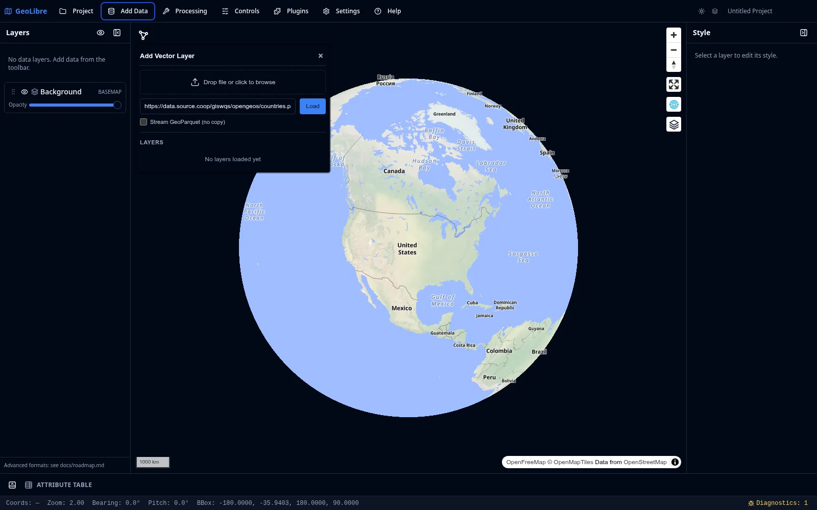
2. In the Add Vector panel, enter a vector URL. You can use the sample countries dataset:
|
|
```text
|
|
https://data.source.coop/giswqs/opengeos/countries.parquet
|
|
```
|
|
3. Click **Load**. The countries appear on the map and a `countries` layer is added to the Layers panel.
|
|
|
|
|
|
|
|
See [Adding Data](../user-guide/adding-data.md) for every supported source.
|
|
|
|
## 3. Style the layer
|
|
|
|
1. Select the `countries` layer in the Layers panel. The [Style panel](../user-guide/styling.md) opens on the right.
|
|
2. Adjust the **Fill color**, **Outline color**, and **Fill opacity** to taste.
|
|
3. To make a choropleth, set **Style type** to **Graduated**, pick a numeric field (for example a population or GDP column), choose a **Colormap**, and click **Apply style type**.
|
|
|
|
## 4. Inspect the data
|
|
|
|
1. Click **Attribute table** on the status bar to expand it, then select the `countries` layer to load its records. See [Attribute Table](../user-guide/attribute-table.md).
|
|
2. Sort by a column, or filter to find a feature. Selecting a row highlights it on the map.
|
|
3. You can also turn on **Identify features** for the layer and click a country on the map to see its attributes in a popup.
|
|
|
|
## 5. Save or share
|
|
|
|
- In the desktop app, use **Project → Save** to write a `.geolibre.json` file.
|
|
- Anywhere, use **Project → Share** to upload the project and get a public link. See [Sharing & Embedding](sharing-embedding.md).
|
|
|
|
## Next steps
|
|
|
|
- Load cloud-native and remote formats in [Cloud-Native Data](cloud-native-data.md).
|
|
- Run geometry tools in [Vector Analysis](vector-analysis.md).
|
|
- Query your data in [Spatial SQL](spatial-sql.md).
|