> [!NOTE]
> 本文档由 WeHub 基于上游 README 翻译整理,属于社区翻译,非官方中文文档。
> [English](./README.en.md) · [原始项目](https://github.com/shap/shap) · [上游 README](https://github.com/shap/shap/blob/HEAD/README.md)
> 原作者、版权与许可证归属以原始项目及本仓库 LICENSE 文件为准。
---
[](https://pypi.org/project/shap/)
[](https://anaconda.org/conda-forge/shap)


[](https://mybinder.org/v2/gh/shap/shap/master)
[](https://shap.readthedocs.io/en/latest/?badge=latest)

[](https://pypi.org/pypi/shap/)
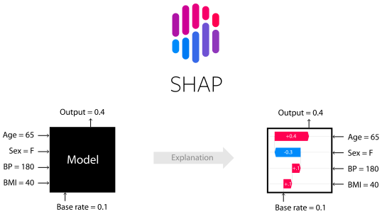
**SHAP (SHapley Additive exPlanations)** 是一种基于博弈论的方法,用于解释任意机器学习模型的输出。它将最优信用分配与局部解释联系起来,采用博弈论中经典的 Shapley 值及其相关扩展(详见 [论文](#citations) 及引用)。
## 安装
可从 [PyPI](https://pypi.org/project/shap) 或 [conda-forge](https://anaconda.org/conda-forge/shap): 安装 SHAP:
pip install shap
or
conda install -c conda-forge shap
### GPU 支持
要启用 GPU 加速的 Tree SHAP,请在已安装 CUDA 工具包且设置 `SHAP_ENABLE_CUDA` 环境变量的情况下从源码安装:
SHAP_ENABLE_CUDA=1 pip install .
这要求你的系统已安装 [CUDA toolkit](https://developer.nvidia.com/cuda-toolkit)。
## 支持的版本
SHAP 遵循 [SPEC 0](https://scientific-python.org/specs/spec-0000/) 规定的最低依赖版本。我们针对其中指定的版本进行测试,可能不会修复旧版本的 bug。
## 贡献
我们非常欢迎贡献。欢迎随时提交 issue。在发起 PR 之前,请确保已阅读我们的 [CONTRIBUTING.md](CONTRIBUTING.md) 指南。
## 树集成示例(XGBoost/LightGBM/CatBoost/scikit-learn/pyspark 模型)
虽然 SHAP 可以解释任意机器学习模型的输出,但我们为树集成方法开发了高速精确算法(参见我们的 [Nature MI 论文](https://rdcu.be/b0z70)). 已为 *XGBoost*、*LightGBM*、*CatBoost*、*scikit-learn* 和 *pyspark* 树模型提供快速 C++ 实现:
```python
import xgboost
import shap
# train an XGBoost model
X, y = shap.datasets.california()
model = xgboost.XGBRegressor().fit(X, y)
# explain the model's predictions using SHAP
# (same syntax works for LightGBM, CatBoost, scikit-learn, transformers, Spark, etc.)
explainer = shap.Explainer(model)
shap_values = explainer(X)
# visualize the first prediction's explanation
shap.plots.waterfall(shap_values[0])
```

上述解释展示了各特征如何将模型输出从基准值(我们传入的训练数据集上模型输出的平均值)推向当前模型输出。使预测值升高的特征显示为红色,使预测值降低的显示为蓝色。可视化同一解释的另一种方式是使用 force plot(在 [Nature BME 论文](https://rdcu.be/baVbR)): 中介绍):
```python
# visualize the first prediction's explanation with a force plot
shap.plots.force(shap_values[0])
```

若将许多如上所示的 force plot 解释旋转 90 度后水平堆叠,即可查看整个数据集的解释(在 notebook 中该图可交互):
```python
# visualize all the training set predictions
shap.plots.force(shap_values[:500])
```

要了解单个特征如何影响模型输出,我们可以绘制该特征的 SHAP 值与数据集中所有样本特征值的对比图。由于 SHAP 值表示某特征对模型输出变化的“责任”,下图展示了预测房价随纬度变化的情况。同一纬度值处的纵向分散表示与其他特征的交互效应。为揭示这些交互,可按另一特征着色。若将整个解释张量传给 `color` 参数,散点图会自动选择最佳着色特征;此处它选择了经度。
```python
# create a dependence scatter plot to show the effect of a single feature across the whole dataset
shap.plots.scatter(shap_values[:, "Latitude"], color=shap_values)
```

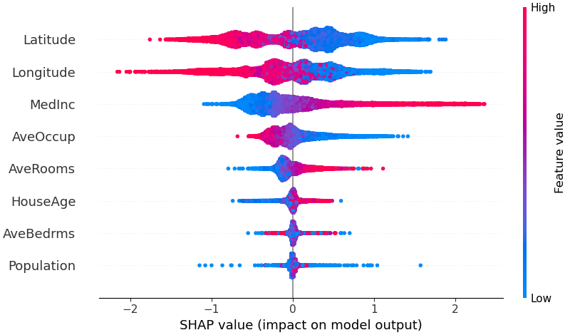
要概览哪些特征对模型最重要,我们可以绘制每个样本每个特征的 SHAP 值。下图按所有样本上 SHAP 值幅度之和对特征排序,并用 SHAP 值展示各特征对模型输出影响的分布。颜色表示特征值(红色为高,蓝色为低)。例如,这揭示了较高的收入中位数会提高预测房价。
```python
# summarize the effects of all the features
shap.plots.beeswarm(shap_values)
```
我们也可以对每个特征 SHAP 值的绝对值取平均,得到标准条形图(多类输出会生成堆叠条形图):
```python
shap.plots.bar(shap_values)
```

## 自然语言示例(transformers)
SHAP 对 Hugging Face transformers 库中的自然语言模型等提供专门支持。通过在传统 Shapley 值上添加联盟规则(coalitional rules),我们可以构造仅需极少函数评估即可解释大型现代 NLP 模型的博弈。使用该功能非常简单,只需将受支持的 transformers pipeline 传给 SHAP:
```python
import transformers
import shap
# load a transformers pipeline model
model = transformers.pipeline('sentiment-analysis', top_k=None)
# explain the model on two sample inputs
explainer = shap.Explainer(model)
shap_values = explainer(["What a great movie! ...if you have no taste."])
# visualize the first prediction's explanation for the POSITIVE output class
shap.plots.text(shap_values[0, :, "POSITIVE"])
```

## 使用 DeepExplainer 的深度学习示例(TensorFlow/Keras 模型)
Deep SHAP 是深度学习模型中 SHAP 值的高速近似算法,建立在 SHAP NIPS 论文中所述与 [DeepLIFT](https://arxiv.org/abs/1704.02685) 的联系之上。此处的实现与原始 DeepLIFT 的不同之处在于:使用背景样本分布而非单一参考值,并使用 Shapley 方程对 max、softmax、乘积、除法等组件进行线性化。请注意,其中一些增强此后也已集成到 DeepLIFT 中。支持 TensorFlow 模型以及使用 TensorFlow 后端的 Keras 模型(对 PyTorch 也有初步支持):
```python
# ...include code from https://github.com/keras-team/keras/blob/master/examples/demo_mnist_convnet.py
import shap
import numpy as np
# select a set of background examples to take an expectation over
background = x_train[np.random.choice(x_train.shape[0], 100, replace=False)]
# explain predictions of the model on four images
e = shap.DeepExplainer(model, background)
# ...or pass tensors directly
# e = shap.DeepExplainer((model.layers[0].input, model.layers[-1].output), background)
shap_values = e.shap_values(x_test[1:5])
# plot the feature attributions
shap.image_plot(shap_values, -x_test[1:5])
```
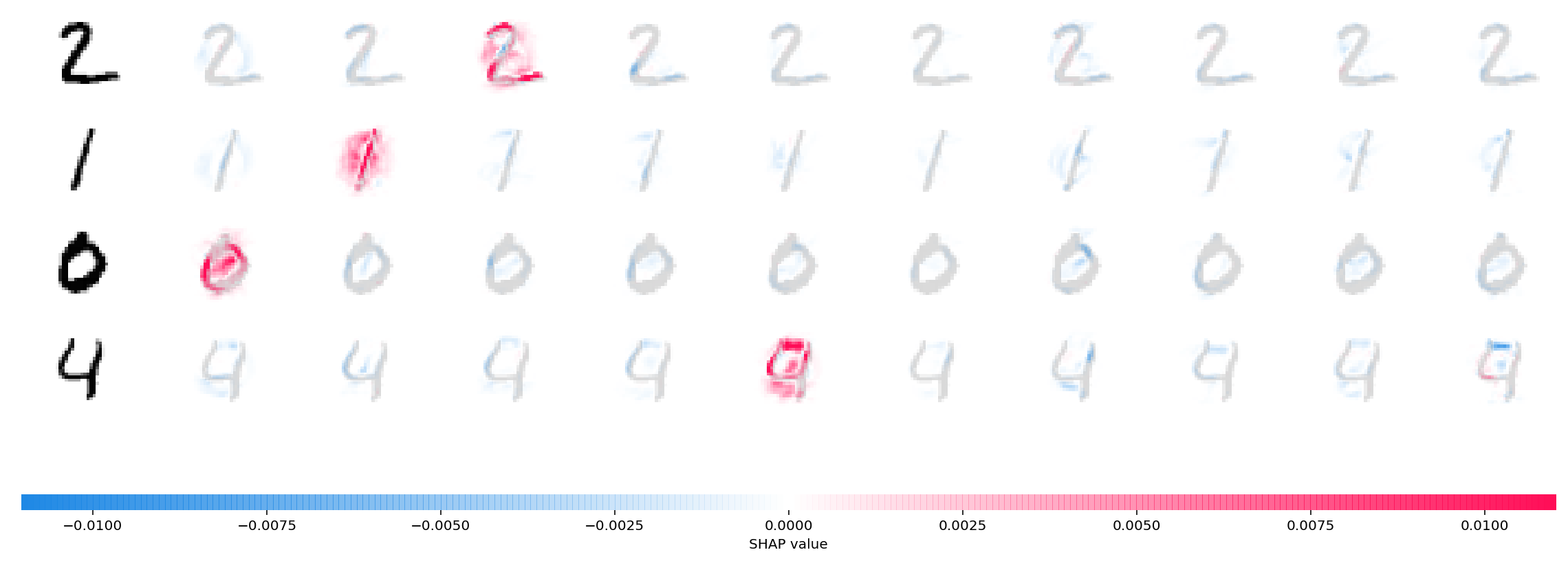
上图解释了四张不同图像对应的十个输出(数字 0-9)。红色像素会提高模型的输出,蓝色像素会降低输出。输入图像显示在左侧,并作为各张解释图背后近乎透明的灰度背景。SHAP 值的总和等于预期模型输出(在背景数据集上取平均)与当前模型输出之间的差值。请注意,对于“零”的图像,中间空白区域很重要;而对于“四”的图像,顶部缺少连接才使它被识别为四而不是九。
## 使用 GradientExplainer 的深度学习示例(TensorFlow/Keras/PyTorch 模型)
Expected gradients(预期梯度)将 [Integrated Gradients](https://arxiv.org/abs/1703.01365), SHAP,以及 [SmoothGrad](https://arxiv.org/abs/1706.03825) 融合到一个单一的期望值方程中。这使得可以将整个数据集用作背景分布(而非单个参考值),并支持局部平滑。若我们用每个背景数据样本与当前待解释输入之间的线性函数来近似模型,并假设输入特征相互独立,则 expected gradients 将计算出近似的 SHAP 值。在下面的示例中,我们解释了 VGG16 ImageNet 模型的第 7 个中间层如何影响输出概率。
```python
from keras.applications.vgg16 import VGG16
from keras.applications.vgg16 import preprocess_input
import keras.backend as K
import numpy as np
import json
import shap
# load pre-trained model and choose two images to explain
model = VGG16(weights='imagenet', include_top=True)
X,y = shap.datasets.imagenet50()
to_explain = X[[39,41]]
# load the ImageNet class names
url = "https://s3.amazonaws.com/deep-learning-models/image-models/imagenet_class_index.json"
fname = shap.datasets.cache(url)
with open(fname) as f:
class_names = json.load(f)
# explain how the input to the 7th layer of the model explains the top two classes
def map2layer(x, layer):
feed_dict = dict(zip([model.layers[0].input], [preprocess_input(x.copy())]))
return K.get_session().run(model.layers[layer].input, feed_dict)
e = shap.GradientExplainer(
(model.layers[7].input, model.layers[-1].output),
map2layer(X, 7),
local_smoothing=0 # std dev of smoothing noise
)
shap_values,indexes = e.shap_values(map2layer(to_explain, 7), ranked_outputs=2)
# get the names for the classes
index_names = np.vectorize(lambda x: class_names[str(x)][1])(indexes)
# plot the explanations
shap.image_plot(shap_values, to_explain, index_names)
```
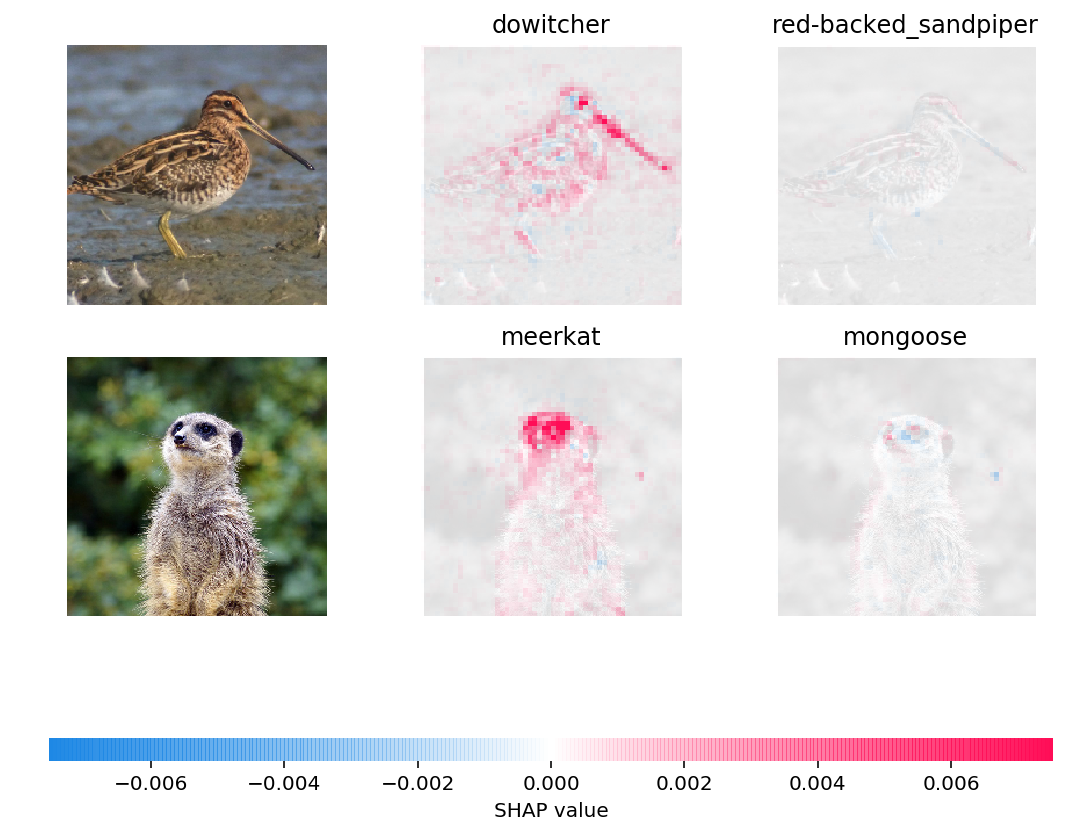
上图解释了两张输入图像的预测结果。红色像素表示正值 SHAP,会提高该类别的概率;蓝色像素表示负值 SHAP,会降低该类别的概率。通过使用 `ranked_outputs=2`,我们仅解释每个输入中最可能的两个类别(这样就不必解释全部 1,000 个类别)。
## 使用 KernelExplainer 的模型无关示例(可解释任意函数)
Kernel SHAP 使用特殊加权的局部线性回归来估计任意模型的 SHAP 值。下面是一个简单示例,用于解释经典 iris 数据集上的多分类 SVM。
```python
import sklearn
import shap
from sklearn.model_selection import train_test_split
# print the JS visualization code to the notebook
shap.initjs()
# train a SVM classifier
X_train,X_test,Y_train,Y_test = train_test_split(*shap.datasets.iris(), test_size=0.2, random_state=0)
svm = sklearn.svm.SVC(kernel='rbf', probability=True)
svm.fit(X_train, Y_train)
# use Kernel SHAP to explain test set predictions
explainer = shap.KernelExplainer(svm.predict_proba, X_train, link="logit")
shap_values = explainer.shap_values(X_test, nsamples=100)
# plot the SHAP values for the Setosa output of the first instance
shap.force_plot(explainer.expected_value[0], shap_values[0][0,:], X_test.iloc[0,:], link="logit")
```

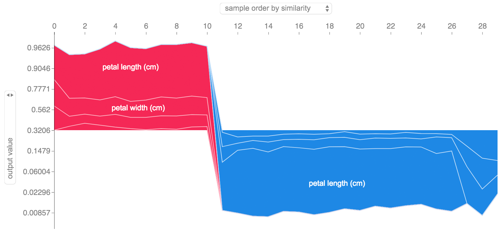
上述解释展示了四个特征各自如何将模型输出从基准值(我们传入的训练数据集上的平均模型输出)推向零。若有任何特征将类别标签推高,则会以红色显示。
若将许多如上所示的解释旋转 90 度,再水平堆叠,便可以看到整个数据集的解释。我们在下面正是这样做的,针对 iris 测试集中的所有样本:
```python
# plot the SHAP values for the Setosa output of all instances
shap.force_plot(explainer.expected_value[0], shap_values[0], X_test, link="logit")
```
## SHAP Interaction Values(SHAP 交互值)
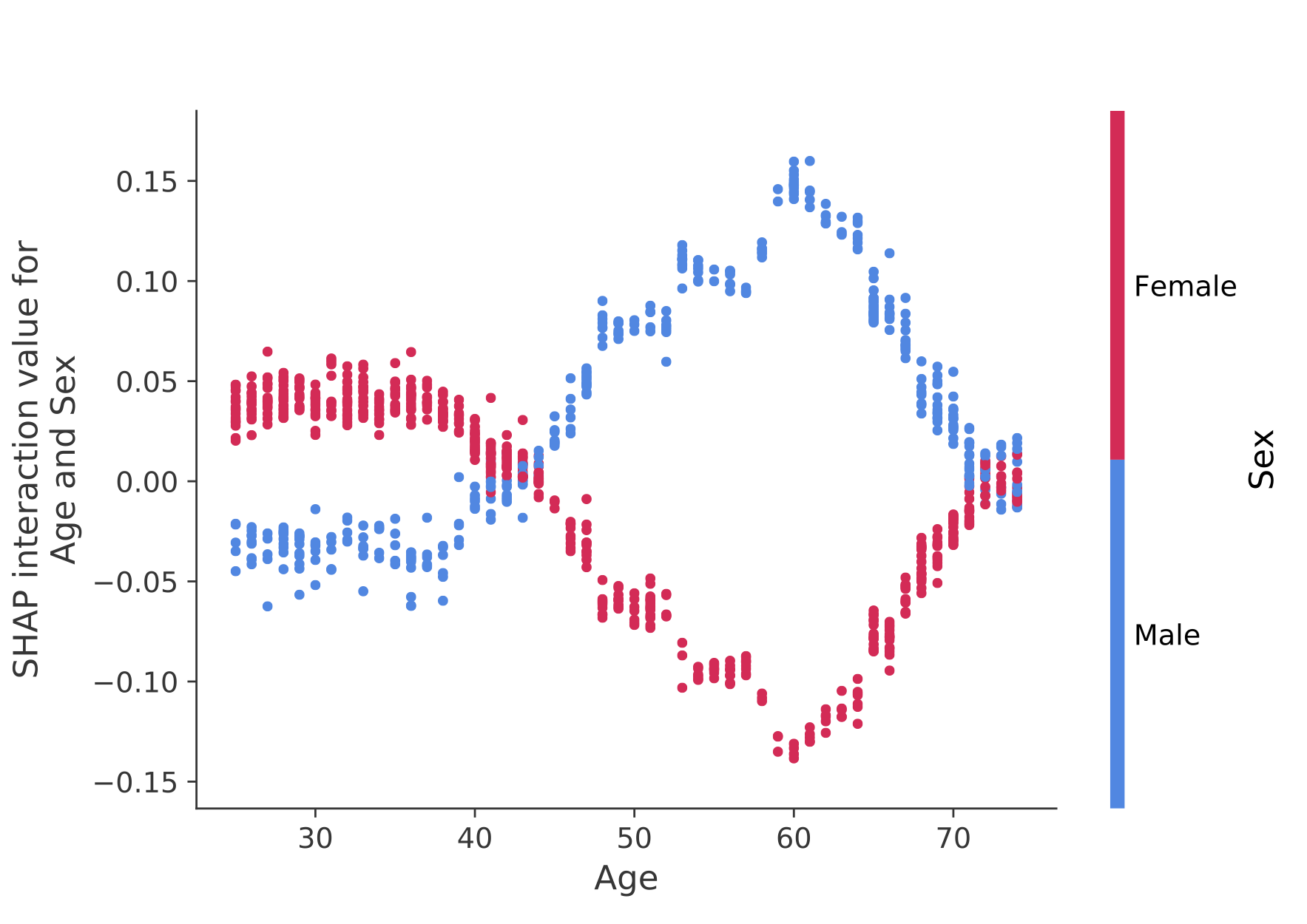
SHAP 交互值是 SHAP 值向高阶交互的推广。对于树模型,已使用 `shap.TreeExplainer(model).shap_interaction_values(X)` 实现了成对交互的快速精确计算。这会为每次预测返回一个矩阵,其中主效应位于对角线,交互效应位于非对角线。这些值常常揭示有趣的隐含关系,例如男性死亡风险在 60 岁时达到峰值(详见 NHANES notebook):
## 示例 notebook
下面的 notebook 演示了 SHAP 的不同使用场景。若想亲自尝试原始 notebook,请查看仓库中的 notebooks 目录。
### TreeExplainer
Tree SHAP 的实现,一种为树及树集成快速精确计算 SHAP 值的算法。
- [**使用 XGBoost 和 SHAP 交互值的 NHANES 生存模型**](https://shap.github.io/shap/notebooks/NHANES%20I%20Survival%20Model.html) - 使用 20 年随访的死亡率数据,该 notebook 演示如何使用 XGBoost 和 `shap` 揭示复杂的风险因素关系。
- [**使用 LightGBM 进行 Census 收入分类**](https://shap.github.io/shap/notebooks/tree_explainer/Census%20income%20classification%20with%20LightGBM.html) - 使用标准的 adult census income 数据集,该 notebook 使用 LightGBM 训练梯度提升树模型,然后使用 `shap` 解释预测结果。
- [**使用 XGBoost 进行 League of Legends 胜负预测**](https://shap.github.io/shap/notebooks/League%20of%20Legends%20Win%20Prediction%20with%20XGBoost.html) - 使用 Kaggle 上 18 万场排位赛的 League of Legends 数据集,我们使用 XGBoost 训练并解释梯度提升树模型,以预测玩家是否会赢得比赛。
### DeepExplainer
Deep SHAP 的实现,一种为深度学习模型计算 SHAP 值的更快(但仅为近似)算法,基于 SHAP 与 DeepLIFT 算法之间的联系。
- [**使用 Keras 进行 MNIST 手写数字分类**](https://shap.github.io/shap/notebooks/deep_explainer/Front%20Page%20DeepExplainer%20MNIST%20Example.html) - 本 notebook 使用 MNIST 手写识别数据集训练 Keras 神经网络,并使用 `shap` 解释预测结果。
- [**使用 Keras LSTM 进行 IMDB 情感分类**](https://shap.github.io/shap/notebooks/deep_explainer/Keras%20LSTM%20for%20IMDB%20Sentiment%20Classification.html) - 本 notebook 在 IMDB 文本情感分析数据集上使用 Keras 训练 LSTM,并使用 `shap` 解释预测结果。
### GradientExplainer
基于期望梯度(expected gradients)来近似深度学习模型 SHAP 值的实现。它建立在 SHAP 与 Integrated Gradients 算法之间的联系之上。GradientExplainer 比 DeepExplainer 更慢,并采用不同的近似假设。
- [**解释 ImageNet 上 VGG16 的中间层**](https://shap.github.io/shap/notebooks/gradient_explainer/Explain%20an%20Intermediate%20Layer%20of%20VGG16%20on%20ImageNet.html) - 本 notebook 演示如何使用内部卷积层来解释预训练 VGG16 ImageNet 模型的输出。
### LinearExplainer
对于特征相互独立的线性模型,我们可以解析地计算精确的 SHAP 值。若愿意估计特征协方差矩阵,也可以考虑特征相关性。LinearExplainer 同时支持这两种选项。
- [**使用逻辑回归进行情感分析**](https://shap.github.io/shap/notebooks/linear_explainer/Sentiment%20Analysis%20with%20Logistic%20Regression.html) - 本 notebook 演示如何解释线性逻辑回归情感分析模型。
### KernelExplainer
Kernel SHAP 的实现,这是一种模型无关(model agnostic)方法,可为任意模型估计 SHAP 值。由于不对模型类型做任何假设,KernelExplainer 比其他针对特定模型类型的算法更慢。
- [**使用 scikit-learn 进行人口普查收入分类**](https://shap.github.io/shap/notebooks/Census%20income%20classification%20with%20scikit-learn.html) - 本 notebook 使用标准 adult 人口普查收入数据集,通过 scikit-learn 训练 k 近邻分类器,并使用 `shap` 解释预测结果。
- [**使用 Keras 的 ImageNet VGG16 模型**](https://shap.github.io/shap/notebooks/ImageNet%20VGG16%20Model%20with%20Keras.html) - 解释经典 VGG16 卷积神经网络对某张图像的预测。该方法将模型无关的 Kernel SHAP 应用于超像素(super-pixel)分割后的图像。
- [**鸢尾花分类**](https://shap.github.io/shap/notebooks/Iris%20classification%20with%20scikit-learn.html) - 使用广为人知的鸢尾花物种数据集进行基础演示。它使用 `shap` 解释 scikit-learn 中六种不同模型的预测结果。
## 文档类 notebook
这些 notebook 全面演示了如何使用特定函数和对象。
- [`shap.decision_plot` 与 `shap.multioutput_decision_plot`](https://shap.github.io/shap/notebooks/plots/decision_plot.html)
- [`shap.dependence_plot`](https://shap.github.io/shap/notebooks/plots/dependence_plot.html)
## 由 SHAP 统一的方法
1. *LIME:* Ribeiro, Marco Tulio, Sameer Singh, and Carlos Guestrin. "Why should i trust you?: Explaining the predictions of any classifier." Proceedings of the 22nd ACM SIGKDD International Conference on Knowledge Discovery and Data Mining. ACM, 2016.
2. *Shapley sampling values:* Strumbelj, Erik, and Igor Kononenko. "Explaining prediction models and individual predictions with feature contributions." Knowledge and information systems 41.3 (2014): 647-665.
3. *DeepLIFT:* Shrikumar, Avanti, Peyton Greenside, and Anshul Kundaje. "Learning important features through propagating activation differences." arXiv preprint arXiv:1704.02685 (2017).
4. *QII:* Datta, Anupam, Shayak Sen, and Yair Zick. "Algorithmic transparency via quantitative input influence: Theory and experiments with learning systems." Security and Privacy (SP), 2016 IEEE Symposium on. IEEE, 2016.
5. *Layer-wise relevance propagation:* Bach, Sebastian, et al. "On pixel-wise explanations for non-linear classifier decisions by layer-wise relevance propagation." PloS one 10.7 (2015): e0130140.
6. *Shapley regression values:* Lipovetsky, Stan, and Michael Conklin. "Analysis of regression in game theory approach." Applied Stochastic Models in Business and Industry 17.4 (2001): 319-330.
7. *Tree interpreter:* Saabas, Ando. Interpreting random forests. http://blog.datadive.net/interpreting-random-forests/
## 引用
本软件包中使用的算法和可视化主要源自 [Su-In Lee 实验室](https://suinlee.cs.washington.edu) 在华盛顿大学以及 Microsoft Research 开展的研究。若您在研究中使用 SHAP,我们希望能引用相应的论文:
- 对于 SHAP 的一般用途,您可以阅读/引用我们的 [NeurIPS 论文](http://papers.nips.cc/paper/7062-a-unified-approach-to-interpreting-model-predictions)([bibtex](https://raw.githubusercontent.com/shap/shap/master/docs/references/shap_nips.bib)).
- 对于 TreeExplainer,您可以阅读/引用我们的 [Nature Machine Intelligence 论文](https://www.nature.com/articles/s42256-019-0138-9)([bibtex](https://raw.githubusercontent.com/shap/shap/master/docs/references/tree_explainer.bib); [免费获取](https://rdcu.be/b0z70)).
- 对于 GPUTreeExplainer,您可以阅读/引用[这篇文章](https://arxiv.org/abs/2010.13972).
- 对于 `force_plot` 可视化及医学应用,您可以阅读/引用我们的 [Nature Biomedical Engineering 论文](https://www.nature.com/articles/s41551-018-0304-0)([bibtex](https://raw.githubusercontent.com/shap/shap/master/docs/references/nature_bme.bib); [免费获取](https://rdcu.be/baVbR)).
