wehub/fareedkhan-dev--train-llm-from-scratch

Fork 0

Files

T

wehub-resource-sync 40c81e098f docs: make Chinese README the default

2026-07-13 10:17:12 +00:00

36 KiB

Raw Blame History

Note

本文档由 WeHub 基于上游 README 翻译整理，属于社区翻译，非官方中文文档。
English · 原始项目 · 上游 README
原作者、版权与许可证归属以原始项目及本仓库 LICENSE 文件为准。

从零训练大语言模型（LLM）

我正在寻找人工智能方向的博士职位。 GitHub

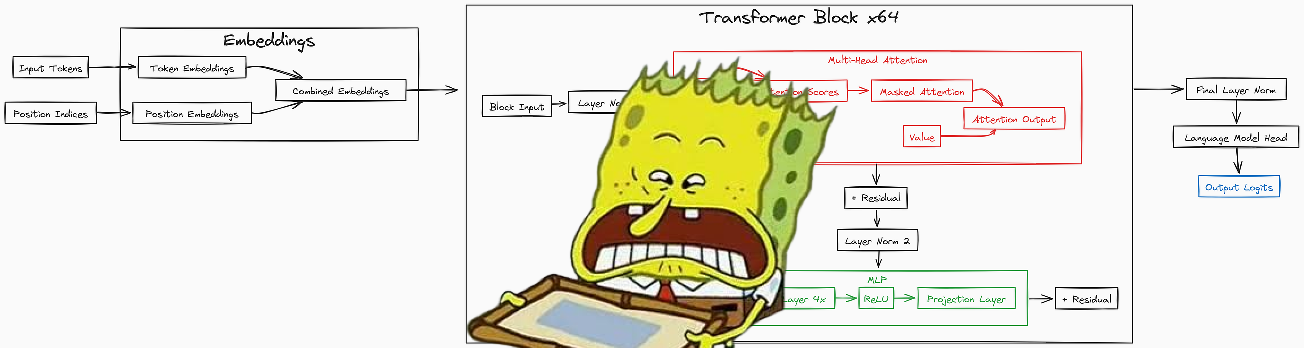
我基于论文 Attention is All You Need. 使用 PyTorch 从零实现了一个 Transformer 模型。你可以用我的脚本在单张 GPU 上训练自己的十亿或百万参数的大语言模型。

这最初是一份预训练教程。现在它涵盖了从原始文本到对齐的、具备推理风格模型的完整流程，每个算法都是用纯 PyTorch 手写的（没有 trl，没有 peft，没有 transformers）。整个旅程重复着一个核心思路：把文本变成数字，预测下一个 token，然后不断调整数据和损失函数，直到模型按我们的期望行事。

下面是我们将端到端走过的路径：

raw text  ->  tokens  ->  a Transformer  ->  next-token loss  ->  a base model
base model  ->  SFT  ->  Reward Model  ->  {PPO, DPO}  ->  GRPO  ->  evaluation and chat

下面是一个训练好的 1300 万参数大语言模型的输出，让你了解这套方法在小型模型端的表现：

In ***1978, The park was returned to the factory-plate that
the public share to the lower of the electronic fence that
follow from the Station's cities. The Canal of ancient Western
nations were confined to the city spot. The villages were directly
linked to cities in China that revolt that the US budget and in
Odambinais is uncertain and fortune established in rural areas.

适用读者
前置要求与训练时间
环境搭建
代码结构
步骤 1：准备数据
步骤 2：由小组件构建模型
步骤 3：预训练基座模型
步骤 4：生成文本
步骤 5：后训练——将基座模型变为助手
步骤 6：评估
步骤 7：与模型对话
Streamlit 控制面板
文档站点
运行完整流程
下一步

适用读者

我尽量让这一页能同时满足不同背景的读者：

如果你是学生，请从上到下阅读。每段代码之前都有通俗说明——它做什么、为什么这样做；大多数代码块之后还附有你应该看到的输出。
如果你是 开发者，所需的命令和文件路径都在这里。你可以直接复制、运行，并阅读引用的源文件。
如果你是 研究者，后训练部分更值得一看：SFT、Bradley-Terry 奖励模型、带 GAE 的 PPO、DPO/ORPO/KTO，以及 GRPO——全部在同一小型 Transformer 上从零实现，并在真实公开数据集上训练。

本 README 中的每张图都采用统一配色，颜色含义如下：

绿色表示原始数据
青色表示磁盘上已存储、已分词的数据
蓝色表示普通处理步骤
黄色表示模型或训练步骤
橙色表示强化学习与奖励相关部分
红色表示损失（loss）
灰色表示已保存的检查点（checkpoint）
紫色表示最终输出或评估

前置要求与训练时间

你需要具备面向对象编程、神经网络和 PyTorch 的基础知识。以下是一些入门资源：

主题	视频链接
OOP（面向对象编程）	OOP Video
Neural Network（神经网络）	Neural Network Video
Pytorch	Pytorch Video

训练需要 GPU。免费的 Colab 或 Kaggle T4 足以训练 1300 万参数模型，但无法容纳十亿参数模型。以下是粗略参考：

GPU 名称	显存	20 亿参数 LLM 训练	1300 万参数 LLM 训练	最大实用 LLM 规模（训练）
NVIDIA A100	40 GB	✔	✔	~6B 至 8B
NVIDIA V100	16 GB	✘	✔	~2B
NVIDIA RTX 4090	24 GB	✔	✔	~4B
NVIDIA RTX 5090	32 GB	✔	✔	1300 万参数已验证，更大配置待定
NVIDIA RTX 3090	24 GB	✔	✔	~3.5B 至 4B
NVIDIA RTX 4080	16 GB	✘	✔	~2B
NVIDIA RTX 4060	8 GB	✘	✔	~1B
Tesla T4	16 GB	✘	✔	~1.5B 至 2B

若大型配置显存不足，预训练脚本提供可选标志（--amp、--grad-checkpointing、--grad-accum），可显著降低显存占用。后续会详细介绍。

环境搭建

克隆仓库并以可编辑模式安装。可编辑安装会把 config、src、data_loader 和 ui 加入导入路径，因此你不再需要手动设置 PYTHONPATH：

git clone https://github.com/FareedKhan-dev/train-llm-from-scratch.git
cd train-llm-from-scratch
pip install -e .

可按需安装可选扩展：

pip install -e ".[train]"   # datasets + wandb, for downloading data and logging
pip install -e ".[ui]"      # streamlit + pandas + altair, for the control panel
pip install -e ".[docs]"    # mkdocs, for the documentation site
pip install -e ".[all]"     # everything

项目有两套配置系统，一开始就分清它们会很有帮助：

config/config.py 是面向旧版预训练脚本 scripts/train_transformer.py 的原始简易配置，采用普通 Python 常量。
config/post_training_config.py 以及 configs/ 中的 JSON 文件驱动其余所有流程（更大基座的预训练、SFT、奖励模型、DPO、PPO、GRPO）。每个阶段编辑一个小 JSON 文件即可，任何字段也可在命令行覆盖，例如 --lr 2e-5 --batch_size 16。

为快速验证，每个阶段都提供精简版 configs/smoke/，会缩小模型规模，使完整运行在 CPU 或单张 GPU 上数秒内完成。

代码结构

train-llm-from-scratch/
├── src/
│   ├── models/                  # the Transformer, built from small pieces
│   │   ├── mlp.py               # the feed-forward block
│   │   ├── attention.py         # single head and multi head attention
│   │   ├── transformer_block.py # one block: attention + MLP + residuals
│   │   └── transformer.py       # the full model: embeddings + blocks + lm_head
│   └── post_training/           # SFT, reward model, PPO, DPO, GRPO, eval, inference
├── config/
│   ├── config.py                # legacy pretraining config (plain constants)
│   ├── post_training_config.py  # dataclasses for every post-training stage
│   └── loader.py                # merges defaults < base.json < stage.json < CLI
├── configs/                     # editable JSON, one file per stage (+ smoke/)
├── data_loader/                 # batch iterators for each kind of data
├── scripts/                     # every runnable step lives here
├── ui/                          # the Streamlit control panel
├── docs/                        # the MkDocs site (theory + diagrams)
├── images/                      # the diagrams in this README (+ the generator)
└── pyproject.toml               # pip install -e .

第 1 步：准备数据

模型看到的只有整数。因此第一步永远是相同的：把文本转成 token id，并以训练时便于快速读取的格式存到磁盘。我们会做四次，对应后面要进行的几类训练。

四条数据流分别是：

来自 The Pile, 的 预训练文本，以 token id 扁平数组形式存储在 HDF5 文件中。
用于 SFT 的 指令数据（Alpaca、Dolly、GSM8K），打包成定长行，并附带掩码标明哪些 token 属于助手的回答。
用于奖励模型和 DPO 的 偏好对（Anthropic HH-RLHF、UltraFeedback），存储为 {prompt, chosen, rejected}。
用于 PPO 和 GRPO 的 RL 提示（GSM8K 及小规模算术热身），存储为 {prompt, gold}。

分词（Tokenization）

我们使用 OpenAI 的 tiktoken 中的 r50k_base 分词器，与 GPT-3 所用相同。文本会变成整数列表，并在每篇文档末尾追加特殊的 <|endoftext|> token（id 50256），以便模型学会一段文本何处结束、下一段何处开始。

旧路径：下载 The Pile 的一个切片并分词为 HDF5：

python scripts/data_download.py            # downloads the validation file + 1 training shard
python scripts/data_preprocess.py          # tokenizes to data/train/pile_train.h5 and data/val/pile_dev.h5

更新、更快的路径会流式读取并批量编码同一数据，直接写入扁平 token 数组：

python scripts/prepare_pretrain_data.py --split val   --out data/pile_dev.h5
python scripts/prepare_pretrain_data.py --split train --num_shards 1 --out data/pile_train.h5

分词完成后，数据就是一长串整数。下面是为此 README 准备的验证文件的真实片段（8.76 million token）：前十个 id，以及它们解码回的内容：

#### OUTPUT ####
dtype: int32 | shape: (8762951,) | total tokens: 8762951
first 10 token ids: [18610, 286, 3993, 3081, 319, 4088, 11, 4640, 2163, 11]
decoded back to text:
'Effect of sleep quality on memory, executive function, and language
 performance in patients with refractory focal epilepsy ...'

这就是分词的核心：输入文本，输出整数扁平数组，而这些整数可直接解码回原文。

对话格式与损失掩码（loss mask）

预训练之后，模型必须知道谁在说话。r50k_base 分词器只有一个特殊 token，因此我们不再发明新 token，而是用纯文本角色标记，让模型在 SFT 中自行学习。单轮对话如下（见 src/post_training/chat_template.py）：

<|user|>
{user content}<|endoftext|><|assistant|>
{assistant content}<|endoftext|>

数学与推理任务中，我们要求助手按固定结构展示推导过程，因为后续强化学习奖励会检查答案标签内的数字：

<think>step by step reasoning ...</think><answer>42</answer>

关键技巧是 loss mask。编码对话时，我们同时构建 0/1 掩码：仅在助手 token（以及结束该轮的 <|endoftext|>）上为 1。这样 SFT 训练的是写回答，而不是复述提示。下面是构建 id 与对齐掩码的代码：

def encode_chat(messages, add_generation_prompt=False):
    ids, mask = [], []
    for m in messages:
        role = m["role"]
        # Role header is always masked out (we never train the model to emit it).
        header_ids = _encode_ordinary(_header_for(role))
        ids.extend(header_ids)
        mask.extend([0] * len(header_ids))

        content_ids = _encode_ordinary(m["content"])
        is_completion = role == "assistant"
        ids.extend(content_ids)
        mask.extend([1 if is_completion else 0] * len(content_ids))   # train on assistant only

        ids.append(EOT_ID)                                            # turn terminator
        mask.append(1 if is_completion else 0)                        # learn to stop
    return ids, mask

下面是本仓库打印的真实渲染对话与验证器奖励示例：

#### OUTPUT ####
rendered chat:
<|user|>
What is 13 + 29?<|endoftext|><|assistant|>
<think>13 + 29 = 42</think><answer>42</answer><|endoftext|>

extract_answer("<answer>42</answer>")        -> 42.0
reward_gsm8k("<answer>42</answer>", 42.0)    -> 1.2    # correct AND well formatted
reward_gsm8k("<answer>7</answer>",  42.0)    -> 0.2    # wrong, but it used the format

下面是一条真实的打包 SFT 行，展示仅助手 token 参与训练（该行 512 个 token 中，掩码为 1 的有 48 个）：

#### OUTPUT ####
tokens shape: (2131, 512) | loss_mask shape: (2131, 512)
row 0: trained (mask=1) tokens = 48 / 512
row 0 decoded:
  <|user|>
  What is the world's oldest annual marathon based on the reference text below? ...
  <|assistant|>
  The Boston Marathon is the world's oldest annual marathon, beginning on April 19th 1897.

各阶段的数据准备脚本如下：

python scripts/prepare_sft_data.py          # Alpaca + Dolly + GSM8K  -> sft_packed.h5
python scripts/prepare_preference_data.py   # HH-RLHF + UltraFeedback -> preferences.jsonl
python scripts/prepare_rl_prompts.py        # GSM8K + arithmetic      -> rl_prompts.jsonl

第 2 步：由小组件组装模型

Transformer 若写成一整块代码会显得吓人，因此我们拆成四个小组件再堆叠。每个组件都是一个小型 nn.Module。我们从最底层开始。

多层感知机（Multi Layer Perceptron，MLP）

MLP 是每个块中负责逐 token「思考」的部分。它接收每个 token 向量，先扩展到四倍维度，施加 ReLU，再压缩回原尺寸。扩展为投影回去之前混合特征留出空间。

class MLP(nn.Module):
    """A simple Multi-Layer Perceptron with one hidden layer."""
    def __init__(self, n_embed):
        super().__init__()
        self.hidden = nn.Linear(n_embed, 4 * n_embed)   # expand to 4x
        self.relu = nn.ReLU()                           # non-linearity
        self.proj = nn.Linear(4 * n_embed, n_embed)     # project back down

    def forward(self, x):
        x = self.relu(self.hidden(x))
        x = self.proj(x)
        return x

__init__ 配置两个线性层与激活函数。forward 按顺序执行它们。输入与输出形状相同，为 (B, T, n_embed)，因此块可直接堆叠而无需变形。代码位于 src/models/mlp.py。

单头注意力（Single Head Attention）

注意力让某个 token 能关注其他 token。每个头从输入构建三种视图：query（我在找什么）、key（我包含什么）、value（若被选中要传递什么）。我们对每个 query 与每个 key 打分，缩放分数，用因果掩码遮蔽未来，经 softmax 将分数变为权重，再对 value 做加权求和。

class Head(nn.Module):
    """A single attention head with causal masking."""
    def __init__(self, head_size, n_embed, context_length):
        super().__init__()
        self.key   = nn.Linear(n_embed, head_size, bias=False)
        self.query = nn.Linear(n_embed, head_size, bias=False)
        self.value = nn.Linear(n_embed, head_size, bias=False)
        # a lower-triangular matrix used to mask out future positions
        self.register_buffer('tril', torch.tril(torch.ones(context_length, context_length)))

    def forward(self, x):
        B, T, C = x.shape
        k = self.key(x)
        q = self.query(x)
        scale_factor = 1 / math.sqrt(C)
        attn_weights = q @ k.transpose(-2, -1) * scale_factor          # (B, T, T) scores
        attn_weights = attn_weights.masked_fill(self.tril[:T, :T] == 0, float('-inf'))  # no peeking ahead
        attn_weights = F.softmax(attn_weights, dim=-1)
        v = self.value(x)
        out = attn_weights @ v                                         # weighted sum of values
        return out

因果掩码（causal mask）正是使其成为语言模型的关键：位置 t 只能关注位置 0..t，而绝不能关注它试图预测的未来。代码位于 src/models/attention.py。

多头注意力（Multi Head Attention）

单个注意力头学习一种关系。我们希望并行运行多个头，以便模型能同时追踪多种模式（例如，代词及其所指的名词）。我们运行 n_head 个注意力头，拼接它们的输出，并将结果再通过一个线性层。

class MultiHeadAttention(nn.Module):
    def __init__(self, n_head, n_embed, context_length):
        super().__init__()
        self.heads = nn.ModuleList(
            [Head(n_embed // n_head, n_embed, context_length) for _ in range(n_head)]
        )
        self.proj = nn.Linear(n_embed, n_embed)   # mixes the heads back together

    def forward(self, x):
        x = torch.cat([h(x) for h in self.heads], dim=-1)   # concat along the feature dim
        x = self.proj(x)
        return x

每个注意力头在大小为 n_embed // n_head 的较小子空间中工作，因此拼接后的结果恰好回到 n_embed。最终的投影层让各个头能够相互通信。

Transformer 块

现在我们将注意力与 MLP 合并为一个块。该块使用 pre-norm 残差连接：我们先做归一化，运行一个子层，再将结果加回输入。这种「加回去」（即残差）使梯度能够流经深层堆叠而不至于消失。

class Block(nn.Module):
    def __init__(self, n_head, n_embed, context_length):
        super().__init__()
        self.ln1 = nn.LayerNorm(n_embed)
        self.attn = MultiHeadAttention(n_head, n_embed, context_length)
        self.ln2 = nn.LayerNorm(n_embed)
        self.mlp = MLP(n_embed)

    def forward(self, x):
        x = x + self.attn(self.ln1(x))   # attention sub-layer + residual
        x = x + self.mlp(self.ln2(x))    # MLP sub-layer + residual
        return x

将 x = x + self.attn(self.ln1(x)) 理解为「关注其他 token，然后将所学内容加回到自身」。MLP 那一行对逐 token 的思考采用同样的思路。代码位于 src/models/transformer_block.py。

完整 Transformer

最后我们将所有部分封装在一起。Token id 通过嵌入表变为向量，我们添加位置嵌入以使模型了解 token 顺序，运行块堆叠，最后再归一化一次，并投影到词汇表大小的分数（称为 logits）。如果传入 targets，模型还会返回交叉熵（cross-entropy）损失。

class Transformer(nn.Module):
    def __init__(self, n_head, n_embed, context_length, vocab_size, N_BLOCKS):
        super().__init__()
        self.token_embed = nn.Embedding(vocab_size, n_embed)
        self.position_embed = nn.Embedding(context_length, n_embed)
        self.attn_blocks = nn.ModuleList(
            [Block(n_head, n_embed, context_length) for _ in range(N_BLOCKS)]
        )
        self.layer_norm = nn.LayerNorm(n_embed)
        self.lm_head = nn.Linear(n_embed, vocab_size)
        self.register_buffer('pos_idxs', torch.arange(context_length))

    def forward(self, idx, targets=None):
        x = self.forward_hidden(idx)        # token + position embeddings, then the blocks + final norm
        logits = self.lm_head(x)            # (B, T, vocab_size)
        loss = None
        if targets is not None:
            B, T, C = logits.shape
            # reshape (not view): the target slice is not contiguous, so .view() fails on CPU
            flat_logits = logits.reshape(B * T, C)
            targets = targets.reshape(B * T).long()
            loss = F.cross_entropy(flat_logits, targets)
        return logits, loss

有一个小细节值得指出：我们在 targets 上使用 .reshape 而非 .view。target 批次是数据的一个非连续切片，而 .view 在 CPU 上无法处理这种情况。.reshape 两种情况都能处理，其他方面完全相同。完整模型（包括 forward_hidden——奖励头与价值头稍后也会复用——以及 generate）位于 src/models/transformer.py。

构建模型时会打印其参数量。本仓库使用的三种规模如下：

#### OUTPUT ####
13M small config (n_embed=128, n_head=8, n_blocks=1):      13,142,656 params
this tutorial's base (n_embed=512, n_head=8, n_blocks=8):  77,031,552 params
post-training default (n_embed=1024, n_head=16, n_blocks=24): 406,359,168 params

第 3 步：预训练基础模型

预训练是最耗时的环节。我们读取随机的 token 窗口，要求模型在每个位置预测下一个 token，用交叉熵衡量其错误程度，并微调权重。我们将此重复数千次。

最简单的版本是原始的 scripts/train_transformer.py，它读取 config/config.py 并在单块 GPU 上训练。要训练 1300 万参数的模型，请在 config/config.py 中设置以下值：

VOCAB_SIZE = 50304
CONTEXT_LENGTH = 128
N_EMBED = 128
N_HEAD = 8
N_BLOCKS = 1

then run:

python scripts/train_transformer.py

对于长时间训练，可以定期保存检查点并在中断后恢复：

python scripts/train_transformer.py --checkpoint-every 1000 --keep-last 3
python scripts/train_transformer.py --resume latest

如果更大的配置无法放入内存，可开启可选的内存节省选项（默认全部关闭，因此默认行为不会改变）：

python scripts/train_transformer.py --amp --grad-checkpointing --grad-accum 8

更大规模的现代路径是 scripts/pretrain_base.py。配方相同，但加入了训练中等规模基础模型所需的要素：跨 GPU 的 DistributedDataParallel、bf16 autocast、梯度累积、带 warmup 的余弦学习率调度，以及定期保存检查点。单 GPU 或多 GPU，命令形式相同：

# one GPU
python scripts/pretrain_base.py
# both GPUs
torchrun --standalone --nproc_per_node=2 scripts/pretrain_base.py

循环的核心很简单。每一步拉取一个批次，在 bf16 下运行前向传播，为梯度累积缩放损失，反向传播，裁剪梯度，并执行优化器步进：

for micro in range(cfg.grad_accum):
    xb, yb = next(batch_iter)
    with amp_autocast(cfg.amp_dtype, ctx.device):
        _, loss = model(xb, yb)
        loss = loss / cfg.grad_accum       # so the accumulated gradient is the full-batch mean
    loss.backward()
torch.nn.utils.clip_grad_norm_(model.parameters(), cfg.grad_clip)
optimizer.step()

训练过程中会打印步数、损失、学习率和吞吐量；在评估时还会打印 dev 损失和峰值 GPU 内存：

#### OUTPUT ####
Model parameters: 77,031,552 (~77M) | world_size=2
Effective batch = 24*4*2 = 192 seqs/step
step 0    | loss 11.1393 | lr 7.50e-06 | 0 tok/s
step 20   | loss 8.6159  | lr 1.57e-04 | 148,936 tok/s
step 100  | loss 6.3108  | lr 6.00e-04 | 150,609 tok/s
  [eval] step 100  | train 6.2501 | dev 6.1745
step 500  | loss 4.5317  | lr 5.39e-04 | 137,334 tok/s
  [eval] step 500  | train 4.7066 | dev 4.6499
step 1000 | loss 4.0100  | lr 3.48e-04 | 131,348 tok/s
  [eval] step 1000 | train 4.1200 | dev 4.1419
step 1500 | loss 3.6483  | lr 1.45e-04 | 123,781 tok/s
  [eval] step 1500 | train 3.8393 | dev 3.8985
step 1900 | loss 3.7725  | lr 6.36e-05 | 151,488 tok/s
  [eval] step 1900 | train 3.7345 | dev 3.7607
Done. Final checkpoint -> /ephemeral/ckpts/base_pretrained.pt

损失曲线

以下是我为本 README 在 2×L40 GPU 上训练的 7700 万参数基础模型的真实训练损失与 dev 损失。损失起始于接近 ln(vocab_size)，约为 10.8（均匀猜测的模型的损失），并随模型学习文本统计规律而下降：

本次运行初始损失为 11.14（略高于均匀猜测基线 ln(50304) = 10.83），在 2000 步后降至约 3.73 训练 / 3.76 验证，在两张 L40 上训练速度约为每秒 130,000 至 150,000 个 token。损失曲线下降，正是预训练（pretraining）的全部故事：模型正慢慢将语言模式压缩进其权重之中。

步骤 4：生成文本

训练好的模型会预测下一个 token 的概率分布。要生成文本，我们从该分布中采样一个 token，将其追加到序列末尾，再把更长的序列送回模型。如此重复，直到得到足够多的 token。

def generate(self, idx, max_new_tokens):
    for _ in range(max_new_tokens):
        idx_cond = idx[:, -self.context_length:]    # never look back further than the context window
        logits, _ = self(idx_cond)
        logits = logits[:, -1, :]                   # only the last position matters for the next token
        probs = F.softmax(logits, dim=-1)
        idx_next = torch.multinomial(probs, num_samples=1)
        idx = torch.cat((idx, idx_next), dim=1)
    return idx

从已保存的检查点运行：

python scripts/generate_text.py --model_path models/transformer_B.pt --input_text "The" --max_new_tokens 100

这个 1300 万参数的模型已经能产出真实词汇和大体正确的语法，这正是从小规模起步令人鼓舞之处。

步骤 5：后训练——将基座模型变成助手

基座模型可以续写文本，却无法按指令行事或有意识地推理。这需要后训练（post-training）。好消息是模型本身始终不变。我们复用完全相同的 Transformer 骨干网络，每个阶段只改两件事：数据和损失函数。

让所有这一切都能装进一个小仓库的关键设计思路是：包装，而非重写。教学用的 Transformer 只增加一个额外方法 forward_hidden，该方法返回 lm_head 之前的隐状态。奖励头、价值头以及所有对数概率计算，都围绕这一个方法组合而成。src/models/ 中无需重写任何内容。

SFT（监督微调，Supervised Fine-Tuning）

SFT 教会基座模型以对话格式作答。它仍是下一个 token 预测，唯有一点不同：损失只对助手 token 计算，使用的是步骤 1 中构建的掩码。

def sft_loss(logits, tokens, loss_mask):
    logits = logits[:, :-1, :]        # predict token t+1 from position t
    targets = tokens[:, 1:]
    mask = loss_mask[:, 1:].to(logits.dtype)

    V = logits.size(-1)
    ce = F.cross_entropy(logits.reshape(-1, V).float(), targets.reshape(-1).long(), reduction="none")
    ce = ce.view(targets.shape) * mask          # zero out the prompt positions
    return ce.sum() / mask.sum().clamp(min=1.0) # average over assistant tokens only

准备数据并训练：

python scripts/prepare_sft_data.py --context_length 1024
torchrun --standalone --nproc_per_node=2 scripts/train_sft.py

损失函数代码在 src/post_training/sft.py，训练器在 scripts/train_sft.py。

奖励模型

要做强化学习，就需要一个数字来衡量答案好坏。获取它的方法之一，是在人类偏好对上训练奖励模型。我们在 SFT 骨干之上加一个小型线性头，从最后一个真实 token 读出一个标量，并用 Bradley-Terry 损失训练，使被选答案的得分始终高于被拒答案。

def bradley_terry_loss(chosen_rewards, rejected_rewards):
    """Mean -log sigmoid(chosen - rejected) over a batch of preference pairs."""
    return -F.logsigmoid(chosen_rewards - rejected_rewards).mean()

python scripts/prepare_preference_data.py --source both
torchrun --standalone --nproc_per_node=2 scripts/train_reward.py

核心指标是偏好准确率（preference accuracy），即留出配对中被模型判为更高分的被选答案所占比例。本次在 7974 对真实偏好对上运行，达到 0.574（高于 0.5 的随机基线）；若使用更大模型和更多数据，该值可升至 0.65 至 0.75。

#### OUTPUT ####
Reward model from sft.pt | 7974 pairs | total_steps=996
  [eval] step 250 | test_acc 0.539 | margin 0.006
  [eval] step 750 | test_acc 0.576 | margin 0.063
Done RM. test_acc 0.574 margin 0.063 -> reward.pt

代码位于 src/post_training/reward_model.py 与 src/post_training/reward_train.py。

DPO、ORPO 与 KTO

DPO 完全跳过奖励模型与 RL 循环。它直接作用于偏好对，比较策略使被选答案（相对于冻结的 SFT 参考副本）比被拒答案更可能的程度。

def dpo_loss(policy_chosen_logps, policy_rejected_logps,
             ref_chosen_logps, ref_rejected_logps, beta=0.1):
    pi_logratios = policy_chosen_logps - policy_rejected_logps
    ref_logratios = ref_chosen_logps - ref_rejected_logps
    logits = pi_logratios - ref_logratios
    loss = -F.logsigmoid(beta * logits).mean()
    return loss, ...

torchrun --standalone --nproc_per_node=2 scripts/train_dpo.py --loss_type dpo
#   --loss_type orpo   reference free, folds SFT and alignment into one stage
#   --loss_type kto    works from an unpaired desirable / undesirable signal

本次运行中，DPO 在留出配对上达到 0.574 的隐式奖励准确率（implicit-reward accuracy），即策略比冻结参考更偏好被选回复的比例。三种目标函数均在 src/post_training/dpo.py 中。

PPO

PPO 是经典的 RLHF 循环。对每个提示，模型生成一个答案（rollout），我们对其评分（用奖励模型或 GSM8K 答案校验器），对偏离参考模型施加按 token 计的小惩罚，用 GAE 估计每个 token 的好坏，再执行若干步裁剪梯度更新。

两个关键组件——优势估计与裁剪策略损失——都很简短：

def ppo_policy_loss(new_logp, old_logp, advantages, mask, clip=0.2):
    ratio = torch.exp(new_logp - old_logp)
    surr1 = ratio * advantages
    surr2 = torch.clamp(ratio, 1.0 - clip, 1.0 + clip) * advantages   # the clip keeps the step small
    loss = -masked_mean(torch.min(surr1, surr2), mask)
    return loss, ...

python scripts/prepare_rl_prompts.py
torchrun --standalone --nproc_per_node=2 scripts/train_ppo.py --reward_source verifier
#   --reward_source rm   to use the trained reward model instead of the answer checker

Actor-critic 通过小型价值头（src/post_training/value_head.py）共享骨干，GAE、裁剪策略损失与裁剪价值损失均在 src/post_training/ppo.py 中。

GRPO / RLVR

GRPO 是 2025 年、DeepSeek-R1 风格的方法。它舍弃价值网络。对每个提示，它采样一整组答案，用可验证奖励（最终数字是否与标准答案一致）评分，并以该组自身的均值与标准差作为基线。某答案的优势，就是它比同组其他答案好多少。

def group_advantages(rewards, group_size, eps=1e-4):
    r = rewards.view(-1, group_size)
    mean = r.mean(dim=1, keepdim=True)
    std = r.std(dim=1, keepdim=True)
    adv = (r - mean) / (std + eps)     # how much better than the rest of my group
    return adv.reshape(-1)

torchrun --standalone --nproc_per_node=2 scripts/train_grpo.py --group_size 8

先运行一段简短算术课程，让模型在面对完整 GSM8K 之前能获得一些非零奖励来学习。组相对优势、裁剪替代目标与 k3 KL 惩罚均在 src/post_training/grpo.py 中。

步骤 6：评估

贯穿所有阶段的单一指标是 greedy（贪心）GSM8K 准确率。我们给模型一道数学题，让它生成回答，从 <answer> 标签中提取数字，并与标准答案核对。

for s in base_pretrained sft dpo ppo grpo; do
  python scripts/eval_post_training.py --ckpt models/$s.pt --label $s --limit 200 --append logs/table.jsonl
done
python scripts/eval_post_training.py --table logs/table.jsonl

这会构建核心对比，让你能在同一坐标轴上追踪每个阶段：Base、SFT、DPO、PPO 和 GRPO，全部使用相同的 greedy decoding（贪心解码）和相同的可验证奖励：解析 <answer> 标签内的数字并与标准答案核对。同一命令可在任意 checkpoint 上运行，因此你可以填入自己运行的表格；基础模型越大、预训练算力越多，这些分数就越高。

SFT 之后的变化

SFT 最明显的效果是行为变化。基础模型只知道如何续写文本，因此当你给它一个问题时，它只会继续写更多文字。SFT 之后，模型学会了对话格式：它会在训练时使用的 <think>...</think><answer>...</answer> 结构内作答，而这正是奖励模型和后续 RL 阶段所优化的结构。这种学到的格式是之后每个阶段所依赖的基础。你可以用 scripts/chat.py 与任意阶段的 checkpoint 对话，直接观察这一点——这正是下一节的内容。

第 7 步：与模型对话

scripts/chat.py 可加载任意 checkpoint，从 checkpoint 自身读取模型维度，并让你与之对话。它对指令模型应用 chat template（对话模板），或将基础模型视为原始续写。

# instruction-tuned models
python scripts/chat.py --ckpt models/sft.pt --prompt "What is 13 + 29?"
python scripts/chat.py --ckpt models/grpo.pt --prompt "..." --greedy
# base model, raw continuation
python scripts/chat.py --ckpt models/base_pretrained.pt --raw --prompt "Once upon a time"
# interactive, no --prompt
python scripts/chat.py --ckpt models/sft.pt

生成复用与训练和评估相同的经过验证的核心，因此你在对话中看到的内容正是 RL 阶段所优化的。采样由 --temperature、--top_p、--top_k 或 --greedy 控制。代码位于 src/post_training/inference.py。

Streamlit 控制面板

如果你更愿意点击而非输入命令，有一个小型控制面板可以启动每个阶段、实时查看 loss、运行评估，并与 checkpoint 对话：

pip install -e ".[ui]"
streamlit run ui/app.py

每个阶段对应一页（Data、Pretrain、SFT、Reward、DPO、PPO、GRPO、Evaluate、Chat），每页都是基于你可手动编辑的同一套 JSON 配置的表单。

文档站点

文档站点为每个阶段提供更深入的说明，包括理论、图示、真实代码以及各指标的含义：

https://fareedkhan-dev.github.io/train-llm-from-scratch/

本地运行：

pip install -e ".[docs]"
mkdocs serve

还有一个 Foundations（基础）章节，讲解本代码假定你已了解的概念（tokenization、decoder-only Transformer、attention、objectives、optimization 和 generation）。

运行完整流程

基础模型完成预训练且数据准备就绪后，一个脚本即可运行整个 post-training（后训练）流程，并打印跨阶段对比表：

bash scripts/run_posttraining.sh            # uses both GPUs via torchrun
NPROC=1 bash scripts/run_posttraining.sh    # single GPU

若要对秒级完成的小模型进行快速端到端检查，每个阶段都提供了 smoke config（冒烟配置）：

python tests/test_post_training_smoke.py                          # core math, on CPU
python scripts/train_sft.py --config configs/smoke/sft.json       # a real (tiny) training run

下一步

我建议你先训练 1300 万参数模型，观察它能产出通顺的词，然后用 memory flags 逐步放大 n_embed 和 n_blocks，直到触及 GPU 上限。之后逐阶段走完 post-training 流程，观察 GSM8K 分数的变化。每个阶段的代码都足够精简，一次通读即可，且它们共用同一套模型。

若想深入了解某个特定阶段，文档站点为每个阶段都设有专题页面。

想聊点什么？My Linkedin

36 KiB

Raw Blame History

从零训练大语言模型（LLM）

目录

适用读者

前置要求与训练时间

环境搭建

代码结构

第 1 步：准备数据

分词（Tokenization）

对话格式与损失掩码（loss mask）

第 2 步：由小组件组装模型

多层感知机（Multi Layer Perceptron，MLP）

单头注意力（Single Head Attention）

多头注意力（Multi Head Attention）

Transformer 块

完整 Transformer

第 3 步：预训练基础模型

损失曲线

步骤 4：生成文本

步骤 5：后训练——将基座模型变成助手

SFT（监督微调，Supervised Fine-Tuning）

奖励模型

DPO、ORPO 与 KTO

PPO

GRPO / RLVR

步骤 6：评估

SFT 之后的变化

第 7 步：与模型对话

Streamlit 控制面板

文档站点

运行完整流程

下一步

Star History

36 KiB Raw Blame History Unescape Escape

从零训练大语言模型（LLM）

目录

适用读者

前置要求与训练时间

环境搭建

代码结构

第 1 步：准备数据

分词（Tokenization）

对话格式与损失掩码（loss mask）

第 2 步：由小组件组装模型

多层感知机（Multi Layer Perceptron，MLP）

单头注意力（Single Head Attention）

多头注意力（Multi Head Attention）

Transformer 块

完整 Transformer

第 3 步：预训练基础模型

损失曲线

步骤 4：生成文本

步骤 5：后训练——将基座模型变成助手

SFT（监督微调，Supervised Fine-Tuning）

奖励模型

DPO、ORPO 与 KTO

PPO

GRPO / RLVR

步骤 6：评估

SFT 之后的变化

第 7 步：与模型对话

Streamlit 控制面板

文档站点

运行完整流程

下一步

Star History

36 KiB

Raw Blame History