# Train LLM From Scratch
   [](https://fareedkhan-dev.github.io/train-llm-from-scratch/)
**I am Looking for a PhD position in AI**. [GitHub](https://github.com/FareedKhan-dev)
I implemented a transformer model from scratch using PyTorch, based on the paper [Attention is All You Need](https://arxiv.org/abs/1706.03762). You can use my scripts to train your own **billion** or **million** parameter LLM using a single GPU.
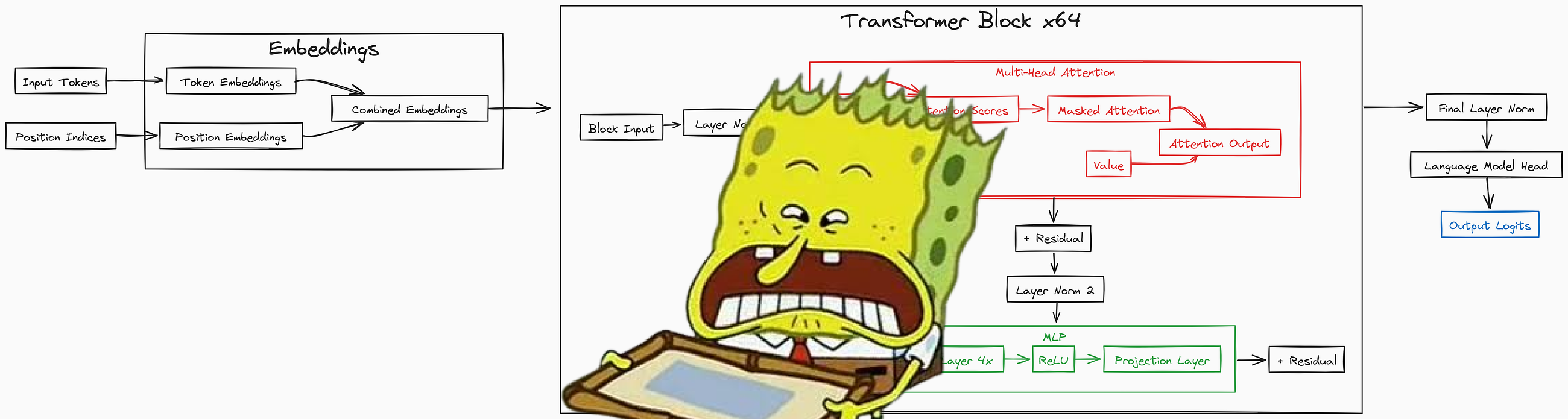
This started as a pretraining tutorial. It now goes all the way from raw text to an aligned, reasoning style model, with every algorithm hand written in plain PyTorch (no `trl`, no `peft`, no `transformers`). The whole journey is one idea repeated: turn text into numbers, predict the next token, then keep changing the data and the loss until the model does what we want.

Here is the path we will walk, end to end:
```
raw text -> tokens -> a Transformer -> next-token loss -> a base model
base model -> SFT -> Reward Model -> {PPO, DPO} -> GRPO -> evaluation and chat
```
Below is the output of a trained 13 million parameter LLM, just so you can see where the small end of this starts:
```
In ***1978, The park was returned to the factory-plate that
the public share to the lower of the electronic fence that
follow from the Station's cities. The Canal of ancient Western
nations were confined to the city spot. The villages were directly
linked to cities in China that revolt that the US budget and in
Odambinais is uncertain and fortune established in rural areas.
```
## Table of Contents
- [Who this is for](#who-this-is-for)
- [Prerequisites and Training Time](#prerequisites-and-training-time)
- [Setup](#setup)
- [Code Structure](#code-structure)
- [Step 1: Preparing the Data](#step-1-preparing-the-data)
- [Step 2: The Model, Built From Small Pieces](#step-2-the-model-built-from-small-pieces)
- [Multi Layer Perceptron (MLP)](#multi-layer-perceptron-mlp)
- [Single Head Attention](#single-head-attention)
- [Multi Head Attention](#multi-head-attention)
- [The Transformer Block](#the-transformer-block)
- [The Full Transformer](#the-full-transformer)
- [Step 3: Pretraining the Base Model](#step-3-pretraining-the-base-model)
- [Step 4: Generating Text](#step-4-generating-text)
- [Step 5: Post-Training, Turning a Base Model Into an Assistant](#step-5-post-training-turning-a-base-model-into-an-assistant)
- [SFT (Supervised Fine-Tuning)](#sft-supervised-fine-tuning)
- [The Reward Model](#the-reward-model)
- [DPO, ORPO and KTO](#dpo-orpo-and-kto)
- [PPO](#ppo)
- [GRPO / RLVR](#grpo--rlvr)
- [Step 6: Evaluation](#step-6-evaluation)
- [Step 7: Talking to the Model](#step-7-talking-to-the-model)
- [The Streamlit Control Panel](#the-streamlit-control-panel)
- [The Documentation Site](#the-documentation-site)
- [Run the Whole Thing](#run-the-whole-thing)
- [What's Next](#whats-next)
## Who this is for
I tried to write this so one page works for very different readers:
- If you are a **student**, read top to bottom. Every block of code comes after a plain explanation of what it does and why, and most blocks are followed by the output you should expect.
- If you are a **developer**, the commands and file paths are all here. You can copy, run, and read the referenced source files directly.
- If you are a **researcher**, the post-training half is the interesting part: SFT, a Bradley-Terry reward model, PPO with GAE, DPO/ORPO/KTO, and GRPO, all from scratch on the same small Transformer, trained on real public datasets.
Every diagram in this README is colored the same way, so the colors mean something:
- green is raw data
- teal is stored, tokenized data on disk
- blue is a plain processing step
- yellow is the model or a training step
- orange is the reinforcement learning and reward parts
- red is a loss
- grey is a saved checkpoint
- purple is the final output or evaluation
## Prerequisites and Training Time
You need a basic understanding of object oriented programming, neural networks, and PyTorch. Below are some resources to help you get started:
| Topic | Video Link |
|---------------------|-----------------------------------------------------------|
| OOP | [OOP Video](https://www.youtube.com/watch?v=Ej_02ICOIgs) |
| Neural Network | [Neural Network Video](https://www.youtube.com/watch?v=Jy4wM2X21u0) |
| Pytorch | [Pytorch Video](https://www.youtube.com/watch?v=V_xro1bcAuA) |
You will need a GPU to train. A free Colab or Kaggle T4 is enough for the 13 million parameter model, but it will not fit a billion parameter model. Here is a rough guide:
| GPU Name | Memory | 2B LLM Training | 13M LLM Training | Max Practical LLM Size (Training) |
|--------------------------|--------|-----------------|------------------|-----------------------------------|
| NVIDIA A100 | 40 GB | ✔ | ✔ | ~6B to 8B |
| NVIDIA V100 | 16 GB | ✘ | ✔ | ~2B |
| NVIDIA RTX 4090 | 24 GB | ✔ | ✔ | ~4B |
| NVIDIA RTX 5090 | 32 GB | ✔ | ✔ | 13M verified, larger configs TBD |
| NVIDIA RTX 3090 | 24 GB | ✔ | ✔ | ~3.5B to 4B |
| NVIDIA RTX 4080 | 16 GB | ✘ | ✔ | ~2B |
| NVIDIA RTX 4060 | 8 GB | ✘ | ✔ | ~1B |
| Tesla T4 | 16 GB | ✘ | ✔ | ~1.5B to 2B |
If a large config runs out of memory, the pretraining script has opt-in flags (`--amp`, `--grad-checkpointing`, `--grad-accum`) that bring the memory down a lot. More on those later.
## Setup
Clone the repository and install it in editable mode. The editable install puts `config`, `src`, `data_loader`, and `ui` on your import path, so you do not need to set `PYTHONPATH` by hand anymore:
```bash
git clone https://github.com/FareedKhan-dev/train-llm-from-scratch.git
cd train-llm-from-scratch
pip install -e .
```
There are optional extras for the parts you want:
```bash
pip install -e ".[train]" # datasets + wandb, for downloading data and logging
pip install -e ".[ui]" # streamlit + pandas + altair, for the control panel
pip install -e ".[docs]" # mkdocs, for the documentation site
pip install -e ".[all]" # everything
```
There are two config systems, and it helps to know which is which from the start:
- `config/config.py` is the original, simple config for the legacy pretraining script `scripts/train_transformer.py`. It is plain Python constants.
- `config/post_training_config.py` plus the JSON files in `configs/` drive everything else (pretraining the bigger base, SFT, reward, DPO, PPO, GRPO). You edit a small JSON file per stage, and any field can also be overridden on the command line, for example `--lr 2e-5 --batch_size 16`.
For fast checks there is a tiny `configs/smoke/` variant of every stage that shrinks the model so a full run finishes in seconds on a CPU or a single GPU.
## Code Structure
```bash
train-llm-from-scratch/
├── src/
│ ├── models/ # the Transformer, built from small pieces
│ │ ├── mlp.py # the feed-forward block
│ │ ├── attention.py # single head and multi head attention
│ │ ├── transformer_block.py # one block: attention + MLP + residuals
│ │ └── transformer.py # the full model: embeddings + blocks + lm_head
│ └── post_training/ # SFT, reward model, PPO, DPO, GRPO, eval, inference
├── config/
│ ├── config.py # legacy pretraining config (plain constants)
│ ├── post_training_config.py # dataclasses for every post-training stage
│ └── loader.py # merges defaults < base.json < stage.json < CLI
├── configs/ # editable JSON, one file per stage (+ smoke/)
├── data_loader/ # batch iterators for each kind of data
├── scripts/ # every runnable step lives here
├── ui/ # the Streamlit control panel
├── docs/ # the MkDocs site (theory + diagrams)
├── images/ # the diagrams in this README (+ the generator)
└── pyproject.toml # pip install -e .
```
## Step 1: Preparing the Data
A model only ever sees integers. So the first job is always the same: take text, turn it into token ids, and store those ids on disk in a format that is fast to read during training. We do this four times, once for each kind of training we will do later.

The four streams are:
1. **Pretraining text** from [The Pile](https://huggingface.co/datasets/monology/pile-uncopyrighted), stored as a flat array of token ids in an HDF5 file.
2. **Instruction data** (Alpaca, Dolly, GSM8K) for SFT, packed into fixed length rows with a mask that says which tokens are the assistant's answer.
3. **Preference pairs** (Anthropic HH-RLHF, UltraFeedback) for the reward model and DPO, stored as `{prompt, chosen, rejected}`.
4. **RL prompts** (GSM8K and a small arithmetic warm-up) for PPO and GRPO, stored as `{prompt, gold}`.
### Tokenization
We use the `r50k_base` tokenizer from OpenAI's `tiktoken`, the same one GPT-3 used. Text becomes a list of integers, and we append a special `<|endoftext|>` token (id 50256) at the end of every document so the model learns where one piece of text stops and the next begins.

For the legacy path, download a slice of The Pile and tokenize it into HDF5:
```bash
python scripts/data_download.py # downloads the validation file + 1 training shard
python scripts/data_preprocess.py # tokenizes to data/train/pile_train.h5 and data/val/pile_dev.h5
```
The newer, faster path streams and batch-encodes the same data straight into a flat token array:
```bash
python scripts/prepare_pretrain_data.py --split val --out data/pile_dev.h5
python scripts/prepare_pretrain_data.py --split train --num_shards 1 --out data/pile_train.h5
```
Once tokenized, the data is just a long line of integers. Here is a real peek at the validation file I prepared for this README (8.76 million tokens), the first ten ids, and what they decode back to:
```python
#### OUTPUT ####
dtype: int32 | shape: (8762951,) | total tokens: 8762951
first 10 token ids: [18610, 286, 3993, 3081, 319, 4088, 11, 4640, 2163, 11]
decoded back to text:
'Effect of sleep quality on memory, executive function, and language
performance in patients with refractory focal epilepsy ...'
```
That is the whole idea of tokenization in one output: text in, a flat array of integers out, and the integers decode straight back to the original words.
### The chat format and loss mask
For everything after pretraining the model has to know who is talking. The `r50k_base` tokenizer has only one special token, so instead of inventing new ones we use plain text role markers that the model simply learns during SFT. A single turn looks like this (see `src/post_training/chat_template.py`):
```
<|user|>
{user content}<|endoftext|><|assistant|>
{assistant content}<|endoftext|>
```
For math and reasoning we ask the assistant to show its work in a fixed structure, because the reinforcement learning reward later checks the number inside the answer tags:
```
step by step reasoning ...42
```
The important trick is the **loss mask**. When we encode a conversation we also build a 0/1 mask that is 1 only on the assistant tokens (and the `<|endoftext|>` that ends the turn). That way SFT trains the model to write answers, not to parrot the prompt back. Here is the exact code that builds the ids and the aligned mask:
```python
def encode_chat(messages, add_generation_prompt=False):
ids, mask = [], []
for m in messages:
role = m["role"]
# Role header is always masked out (we never train the model to emit it).
header_ids = _encode_ordinary(_header_for(role))
ids.extend(header_ids)
mask.extend([0] * len(header_ids))
content_ids = _encode_ordinary(m["content"])
is_completion = role == "assistant"
ids.extend(content_ids)
mask.extend([1 if is_completion else 0] * len(content_ids)) # train on assistant only
ids.append(EOT_ID) # turn terminator
mask.append(1 if is_completion else 0) # learn to stop
return ids, mask
```
Here is a real rendered conversation and the verifier reward in action, printed from this repo:
```python
#### OUTPUT ####
rendered chat:
<|user|>
What is 13 + 29?<|endoftext|><|assistant|>
13 + 29 = 4242<|endoftext|>
extract_answer("42") -> 42.0
reward_gsm8k("42", 42.0) -> 1.2 # correct AND well formatted
reward_gsm8k("7", 42.0) -> 0.2 # wrong, but it used the format
```
And here is one real packed SFT row, showing how only the assistant tokens are trained (the mask is 1 on 48 of the 512 tokens in this row):
```python
#### OUTPUT ####
tokens shape: (2131, 512) | loss_mask shape: (2131, 512)
row 0: trained (mask=1) tokens = 48 / 512
row 0 decoded:
<|user|>
What is the world's oldest annual marathon based on the reference text below? ...
<|assistant|>
The Boston Marathon is the world's oldest annual marathon, beginning on April 19th 1897.
```
The data prep scripts for these stages are:
```bash
python scripts/prepare_sft_data.py # Alpaca + Dolly + GSM8K -> sft_packed.h5
python scripts/prepare_preference_data.py # HH-RLHF + UltraFeedback -> preferences.jsonl
python scripts/prepare_rl_prompts.py # GSM8K + arithmetic -> rl_prompts.jsonl
```
## Step 2: The Model, Built From Small Pieces
A Transformer looks scary as one block of code, so we build it from four small pieces and then stack them. Each piece is a tiny `nn.Module`. We start at the bottom.
### Multi Layer Perceptron (MLP)
The MLP is the part of each block that does the per-token "thinking". It takes each token vector, expands it to four times its size, applies a `ReLU`, and squeezes it back down. The expansion gives the layer room to mix features before projecting back.

```python
class MLP(nn.Module):
"""A simple Multi-Layer Perceptron with one hidden layer."""
def __init__(self, n_embed):
super().__init__()
self.hidden = nn.Linear(n_embed, 4 * n_embed) # expand to 4x
self.relu = nn.ReLU() # non-linearity
self.proj = nn.Linear(4 * n_embed, n_embed) # project back down
def forward(self, x):
x = self.relu(self.hidden(x))
x = self.proj(x)
return x
```
The `__init__` sets up the two linear layers and the activation. The `forward` runs them in order. Input and output shapes are the same, `(B, T, n_embed)`, so blocks can be stacked without any reshaping. The code is in `src/models/mlp.py`.
### Single Head Attention
Attention is the part that lets a token look at other tokens. Each head builds three views of the input: a query (what am I looking for), a key (what do I contain), and a value (what I will pass on if chosen). We score every query against every key, scale the scores, hide the future with a causal mask, turn the scores into weights with a softmax, and take a weighted sum of the values.

```python
class Head(nn.Module):
"""A single attention head with causal masking."""
def __init__(self, head_size, n_embed, context_length):
super().__init__()
self.key = nn.Linear(n_embed, head_size, bias=False)
self.query = nn.Linear(n_embed, head_size, bias=False)
self.value = nn.Linear(n_embed, head_size, bias=False)
# a lower-triangular matrix used to mask out future positions
self.register_buffer('tril', torch.tril(torch.ones(context_length, context_length)))
def forward(self, x):
B, T, C = x.shape
k = self.key(x)
q = self.query(x)
scale_factor = 1 / math.sqrt(C)
attn_weights = q @ k.transpose(-2, -1) * scale_factor # (B, T, T) scores
attn_weights = attn_weights.masked_fill(self.tril[:T, :T] == 0, float('-inf')) # no peeking ahead
attn_weights = F.softmax(attn_weights, dim=-1)
v = self.value(x)
out = attn_weights @ v # weighted sum of values
return out
```
The causal mask is what makes this a language model: position `t` can only attend to positions `0..t`, never to the future it is trying to predict. The code is in `src/models/attention.py`.
### Multi Head Attention
One head learns one kind of relationship. We want many, running in parallel, so the model can track several patterns at once (for example, a pronoun and the noun it refers to). We run `n_head` heads, concatenate their outputs, and pass the result through one more linear layer.

```python
class MultiHeadAttention(nn.Module):
def __init__(self, n_head, n_embed, context_length):
super().__init__()
self.heads = nn.ModuleList(
[Head(n_embed // n_head, n_embed, context_length) for _ in range(n_head)]
)
self.proj = nn.Linear(n_embed, n_embed) # mixes the heads back together
def forward(self, x):
x = torch.cat([h(x) for h in self.heads], dim=-1) # concat along the feature dim
x = self.proj(x)
return x
```
Each head works in a smaller subspace of size `n_embed // n_head`, so the concatenation lands right back at `n_embed`. The final projection lets the heads talk to each other.
### The Transformer Block
Now we combine attention and the MLP into one block. The block uses pre-norm residual connections: we normalize, run a sub-layer, and add the result back to the input. The "add back" (the residual) is what lets gradients flow through a deep stack without vanishing.

```python
class Block(nn.Module):
def __init__(self, n_head, n_embed, context_length):
super().__init__()
self.ln1 = nn.LayerNorm(n_embed)
self.attn = MultiHeadAttention(n_head, n_embed, context_length)
self.ln2 = nn.LayerNorm(n_embed)
self.mlp = MLP(n_embed)
def forward(self, x):
x = x + self.attn(self.ln1(x)) # attention sub-layer + residual
x = x + self.mlp(self.ln2(x)) # MLP sub-layer + residual
return x
```
Read `x = x + self.attn(self.ln1(x))` as "look at the other tokens, then add what you learned back onto yourself". The MLP line is the same idea for the per-token thinking. The code is in `src/models/transformer_block.py`.
### The Full Transformer
Finally we wrap everything. Token ids become vectors through an embedding table, we add a position embedding so the model knows token order, we run the stack of blocks, normalize one last time, and project to vocabulary-sized scores called logits. If we pass targets, the model also returns the cross-entropy loss.

```python
class Transformer(nn.Module):
def __init__(self, n_head, n_embed, context_length, vocab_size, N_BLOCKS):
super().__init__()
self.token_embed = nn.Embedding(vocab_size, n_embed)
self.position_embed = nn.Embedding(context_length, n_embed)
self.attn_blocks = nn.ModuleList(
[Block(n_head, n_embed, context_length) for _ in range(N_BLOCKS)]
)
self.layer_norm = nn.LayerNorm(n_embed)
self.lm_head = nn.Linear(n_embed, vocab_size)
self.register_buffer('pos_idxs', torch.arange(context_length))
def forward(self, idx, targets=None):
x = self.forward_hidden(idx) # token + position embeddings, then the blocks + final norm
logits = self.lm_head(x) # (B, T, vocab_size)
loss = None
if targets is not None:
B, T, C = logits.shape
# reshape (not view): the target slice is not contiguous, so .view() fails on CPU
flat_logits = logits.reshape(B * T, C)
targets = targets.reshape(B * T).long()
loss = F.cross_entropy(flat_logits, targets)
return logits, loss
```
One small detail worth pointing out: we use `.reshape` and not `.view` on the targets. The target batch is a non-contiguous slice of the data, and `.view` refuses to work on that on CPU. `.reshape` handles both cases and is identical in every other way. The full model, including `forward_hidden` (which the reward and value heads reuse later) and `generate`, lives in `src/models/transformer.py`.
When we build the model it prints its parameter count. Here are the three sizes used in this repo:
```python
#### OUTPUT ####
13M small config (n_embed=128, n_head=8, n_blocks=1): 13,142,656 params
this tutorial's base (n_embed=512, n_head=8, n_blocks=8): 77,031,552 params
post-training default (n_embed=1024, n_head=16, n_blocks=24): 406,359,168 params
```
## Step 3: Pretraining the Base Model
Pretraining is the long pole. We read random windows of tokens, ask the model to predict the next token at every position, measure how wrong it was with cross-entropy, and nudge the weights. We repeat that a few thousand times.

The simplest version is the original `scripts/train_transformer.py`, which reads `config/config.py` and trains on one GPU. To train the 13 million parameter model, set these values in `config/config.py`:
```python
VOCAB_SIZE = 50304
CONTEXT_LENGTH = 128
N_EMBED = 128
N_HEAD = 8
N_BLOCKS = 1
```
then run:
```bash
python scripts/train_transformer.py
```
For long runs you can save periodic checkpoints and resume after an interruption:
```bash
python scripts/train_transformer.py --checkpoint-every 1000 --keep-last 3
python scripts/train_transformer.py --resume latest
```
If a bigger config does not fit in memory, turn on the opt-in memory savers (all off by default, so default behavior never changes):
```bash
python scripts/train_transformer.py --amp --grad-checkpointing --grad-accum 8
```
The bigger, modern path is `scripts/pretrain_base.py`. It is the same recipe with the things you need to train a mid-size base: DistributedDataParallel across GPUs, bf16 autocast, gradient accumulation, a cosine learning-rate schedule with warmup, and periodic checkpoints. One GPU or many, same command shape:
```bash
# one GPU
python scripts/pretrain_base.py
# both GPUs
torchrun --standalone --nproc_per_node=2 scripts/pretrain_base.py
```
The core of the loop is small. Each step pulls a batch, runs the forward pass under bf16, scales the loss for gradient accumulation, backpropagates, clips the gradient, and steps the optimizer:
```python
for micro in range(cfg.grad_accum):
xb, yb = next(batch_iter)
with amp_autocast(cfg.amp_dtype, ctx.device):
_, loss = model(xb, yb)
loss = loss / cfg.grad_accum # so the accumulated gradient is the full-batch mean
loss.backward()
torch.nn.utils.clip_grad_norm_(model.parameters(), cfg.grad_clip)
optimizer.step()
```
While it trains it prints the step, the loss, the learning rate, and the throughput, and at eval time it also prints the dev loss and peak GPU memory:
```
#### OUTPUT ####
Model parameters: 77,031,552 (~77M) | world_size=2
Effective batch = 24*4*2 = 192 seqs/step
step 0 | loss 11.1393 | lr 7.50e-06 | 0 tok/s
step 20 | loss 8.6159 | lr 1.57e-04 | 148,936 tok/s
step 100 | loss 6.3108 | lr 6.00e-04 | 150,609 tok/s
[eval] step 100 | train 6.2501 | dev 6.1745
step 500 | loss 4.5317 | lr 5.39e-04 | 137,334 tok/s
[eval] step 500 | train 4.7066 | dev 4.6499
step 1000 | loss 4.0100 | lr 3.48e-04 | 131,348 tok/s
[eval] step 1000 | train 4.1200 | dev 4.1419
step 1500 | loss 3.6483 | lr 1.45e-04 | 123,781 tok/s
[eval] step 1500 | train 3.8393 | dev 3.8985
step 1900 | loss 3.7725 | lr 6.36e-05 | 151,488 tok/s
[eval] step 1900 | train 3.7345 | dev 3.7607
Done. Final checkpoint -> /ephemeral/ckpts/base_pretrained.pt
```
### The loss curve
Here is the real training and dev loss for the 77 million parameter base I trained for this README on 2x L40 GPUs. The loss starts near `ln(vocab_size)`, which is about 10.8 (the loss of a model that guesses uniformly), and drops as the model learns the statistics of the text:

This run started at a loss of **11.14** (just above the uniform-guess line at `ln(50304) = 10.83`) and came down to about **3.73 train / 3.76 dev** after 2000 steps, training at roughly **130,000 to 150,000 tokens per second** across the two L40s. The curve going down is the whole story of pretraining: the model is slowly compressing the patterns of language into its weights.
## Step 4: Generating Text
A trained model predicts a distribution over the next token. To generate, we sample one token from that distribution, append it, and feed the longer sequence back in. We repeat until we have enough tokens.
```python
def generate(self, idx, max_new_tokens):
for _ in range(max_new_tokens):
idx_cond = idx[:, -self.context_length:] # never look back further than the context window
logits, _ = self(idx_cond)
logits = logits[:, -1, :] # only the last position matters for the next token
probs = F.softmax(logits, dim=-1)
idx_next = torch.multinomial(probs, num_samples=1)
idx = torch.cat((idx, idx_next), dim=1)
return idx
```
Run it from a saved checkpoint:
```bash
python scripts/generate_text.py --model_path models/transformer_B.pt --input_text "The" --max_new_tokens 100
```
The 13 million parameter model already produces real words and roughly correct grammar, which is the encouraging part of starting small.
## Step 5: Post-Training, Turning a Base Model Into an Assistant
A base model can continue text, but it cannot follow instructions or reason on purpose. That takes post-training. The good news is that the model never changes. We reuse the exact same Transformer backbone and only change two things at each stage: the data, and the loss.

The one design idea that makes all of this fit in a small repo is **wrap, do not rewrite**. The educational `Transformer` gains a single extra method, `forward_hidden`, which returns the hidden states right before `lm_head`. The reward head, the value head, and all the log-probability math compose around that one method. Nothing in `src/models/` had to be rewritten.
### SFT (Supervised Fine-Tuning)
SFT teaches the base model to answer in the chat format. It is still next-token prediction, with one change: the loss is only counted on the assistant tokens, using the mask we built back in Step 1.

```python
def sft_loss(logits, tokens, loss_mask):
logits = logits[:, :-1, :] # predict token t+1 from position t
targets = tokens[:, 1:]
mask = loss_mask[:, 1:].to(logits.dtype)
V = logits.size(-1)
ce = F.cross_entropy(logits.reshape(-1, V).float(), targets.reshape(-1).long(), reduction="none")
ce = ce.view(targets.shape) * mask # zero out the prompt positions
return ce.sum() / mask.sum().clamp(min=1.0) # average over assistant tokens only
```
Prepare the data and train:
```bash
python scripts/prepare_sft_data.py --context_length 1024
torchrun --standalone --nproc_per_node=2 scripts/train_sft.py
```
The loss code is in `src/post_training/sft.py`, the trainer in `scripts/train_sft.py`.
### The Reward Model
To do reinforcement learning we need a number that says how good an answer is. One way to get it is to train a reward model on human preference pairs. We put a small linear head on top of the SFT backbone that reads one scalar off the last real token, and we train it with the Bradley-Terry loss so the chosen answer always scores higher than the rejected one.

```python
def bradley_terry_loss(chosen_rewards, rejected_rewards):
"""Mean -log sigmoid(chosen - rejected) over a batch of preference pairs."""
return -F.logsigmoid(chosen_rewards - rejected_rewards).mean()
```
```bash
python scripts/prepare_preference_data.py --source both
torchrun --standalone --nproc_per_node=2 scripts/train_reward.py
```
The headline metric is preference accuracy, the fraction of held-out pairs where the model scores the chosen answer higher. In this run on 7974 real preference pairs it reached **0.574** (above the 0.5 chance line); with a larger model and more data this climbs toward 0.65 to 0.75.
```
#### OUTPUT ####
Reward model from sft.pt | 7974 pairs | total_steps=996
[eval] step 250 | test_acc 0.539 | margin 0.006
[eval] step 750 | test_acc 0.576 | margin 0.063
Done RM. test_acc 0.574 margin 0.063 -> reward.pt
```
The code is in `src/post_training/reward_model.py` and `src/post_training/reward_train.py`.
### DPO, ORPO and KTO
DPO skips the reward model and the RL loop entirely. It works directly on preference pairs by comparing how much more likely the policy makes the chosen answer (relative to a frozen reference copy of the SFT model) than the rejected one.

```python
def dpo_loss(policy_chosen_logps, policy_rejected_logps,
ref_chosen_logps, ref_rejected_logps, beta=0.1):
pi_logratios = policy_chosen_logps - policy_rejected_logps
ref_logratios = ref_chosen_logps - ref_rejected_logps
logits = pi_logratios - ref_logratios
loss = -F.logsigmoid(beta * logits).mean()
return loss, ...
```
```bash
torchrun --standalone --nproc_per_node=2 scripts/train_dpo.py --loss_type dpo
# --loss_type orpo reference free, folds SFT and alignment into one stage
# --loss_type kto works from an unpaired desirable / undesirable signal
```
In this run, DPO reached an implicit-reward accuracy of **0.574** on the held-out pairs (the fraction where the policy prefers the chosen response more than the frozen reference does). All three objectives are in `src/post_training/dpo.py`.
### PPO
PPO is the classic RLHF loop. For each prompt the model writes an answer (a rollout), we score it (with the reward model or with a GSM8K answer checker), add a small per-token penalty for drifting away from the reference model, estimate how good each token was with GAE, and take a few clipped gradient steps.

The two load-bearing pieces, the advantage estimate and the clipped policy loss, are short:
```python
def ppo_policy_loss(new_logp, old_logp, advantages, mask, clip=0.2):
ratio = torch.exp(new_logp - old_logp)
surr1 = ratio * advantages
surr2 = torch.clamp(ratio, 1.0 - clip, 1.0 + clip) * advantages # the clip keeps the step small
loss = -masked_mean(torch.min(surr1, surr2), mask)
return loss, ...
```
```bash
python scripts/prepare_rl_prompts.py
torchrun --standalone --nproc_per_node=2 scripts/train_ppo.py --reward_source verifier
# --reward_source rm to use the trained reward model instead of the answer checker
```
The actor-critic shares the backbone through a small value head (`src/post_training/value_head.py`), and the GAE, clipped policy loss, and clipped value loss are in `src/post_training/ppo.py`.
### GRPO / RLVR
GRPO is the 2025, DeepSeek-R1 style method. It throws away the value network. For each prompt it samples a whole group of answers, scores them with a verifiable reward (did the final number match the gold answer), and uses the group's own mean and standard deviation as the baseline. The advantage of an answer is just how much better it did than its group.

```python
def group_advantages(rewards, group_size, eps=1e-4):
r = rewards.view(-1, group_size)
mean = r.mean(dim=1, keepdim=True)
std = r.std(dim=1, keepdim=True)
adv = (r - mean) / (std + eps) # how much better than the rest of my group
return adv.reshape(-1)
```
```bash
torchrun --standalone --nproc_per_node=2 scripts/train_grpo.py --group_size 8
```
A short arithmetic curriculum runs first, so the model gets some non-zero reward to learn from before it faces full GSM8K. The group-relative advantage, the clipped surrogate, and the k3 KL penalty are in `src/post_training/grpo.py`.
## Step 6: Evaluation
The single number that ties all the stages together is greedy GSM8K accuracy. We give the model a math question, let it generate, pull the number out of the `` tags, and check it against the gold answer.

```bash
for s in base_pretrained sft dpo ppo grpo; do
python scripts/eval_post_training.py --ckpt models/$s.pt --label $s --limit 200 --append logs/table.jsonl
done
python scripts/eval_post_training.py --table logs/table.jsonl
```
This builds the headline comparison so you can track every stage on one axis, Base, SFT, DPO, PPO, and GRPO, all with the same greedy decoding and the same verifiable reward: parse the number inside the `` tags and check it against the gold answer. The same command runs on any checkpoint, so you fill in the table for your own run, and the bigger the base model and the more pretraining compute you give it, the higher these scores go.
### What changes after SFT
The clearest effect of SFT is a change in behavior. The base model only knows how to continue text, so when you give it a question it just writes more text. After SFT the model has learned the chat format: it answers inside the `......` structure it was trained on, which is exactly the structure the reward model and the RL stages then optimize against. That learned format is the foundation every stage after it builds on. You can talk to any stage's checkpoint with `scripts/chat.py` and watch this directly, which is the next section.
## Step 7: Talking to the Model
`scripts/chat.py` loads any checkpoint, reads the model dimensions from the checkpoint itself, and lets you talk to it. It applies the chat template for instruction models, or treats the base model as raw continuation.

```bash
# instruction-tuned models
python scripts/chat.py --ckpt models/sft.pt --prompt "What is 13 + 29?"
python scripts/chat.py --ckpt models/grpo.pt --prompt "..." --greedy
# base model, raw continuation
python scripts/chat.py --ckpt models/base_pretrained.pt --raw --prompt "Once upon a time"
# interactive, no --prompt
python scripts/chat.py --ckpt models/sft.pt
```
Generation reuses the same tested core as training and eval, so what you see in chat is exactly what the RL stages optimized. Sampling is controlled by `--temperature`, `--top_p`, `--top_k`, or `--greedy`. The code is in `src/post_training/inference.py`.
## The Streamlit Control Panel
If you would rather click than type, there is a small control panel that can launch every stage, watch the loss live, run evaluation, and chat with a checkpoint:
```bash
pip install -e ".[ui]"
streamlit run ui/app.py
```
It has one page per stage (Data, Pretrain, SFT, Reward, DPO, PPO, GRPO, Evaluate, Chat), each one a form over the same JSON configs you would edit by hand.
## The Documentation Site
Every stage has a deeper write-up, with the theory, the diagram, the real code, and what each metric means, on the documentation site:
**https://fareedkhan-dev.github.io/train-llm-from-scratch/**
To run it locally:
```bash
pip install -e ".[docs]"
mkdocs serve
```
There is also a Foundations section that explains the ideas this code assumes you know (tokenization, the decoder-only Transformer, attention, objectives, optimization, and generation).
## Run the Whole Thing
Once the base is pretrained and the data is prepared, one script runs the entire post-training chain and prints the across-stages table:
```bash
bash scripts/run_posttraining.sh # uses both GPUs via torchrun
NPROC=1 bash scripts/run_posttraining.sh # single GPU
```
For a fast end-to-end check on a tiny model that finishes in seconds, every stage has a smoke config:
```bash
python tests/test_post_training_smoke.py # core math, on CPU
python scripts/train_sft.py --config configs/smoke/sft.json # a real (tiny) training run
```
## What's Next
I recommend you start by training the 13 million parameter model, see it produce sensible words, then scale `n_embed` and `n_blocks` up with the memory flags until you hit your GPU limit. After that, walk the post-training chain one stage at a time and watch the GSM8K number move. Every stage is small enough to read in one sitting, and they all share the same model.
If you want to go deeper on any single stage, the documentation site has a focused page for each one.
Wanna chat on something? [My Linkedin](https://www.linkedin.com/in/fareed-khan-dev/)
## Star History
[](https://star-history.com/#FareedKhan-dev/train-llm-from-scratch&Date)